|
|
1.IntroductionLow concentration, holographic planar concentrator (HPC) technology has been shown to reduce the amount of silicon photovoltaic (PV) material needed in a solar panel.1, 2, 3 Due to the significantly reduced cost of the holographic elements, the HPC panel has an overall reduced costs per watt,1, 2, 3 the tradeoff being that the HPC panel operates at a lower overall area efficiency than a conventionally built PV panel. The results presented in this work, both experimental and theoretical, show that the addition of the holographic regions in the areas next to the silicon cell sections creates a larger surface for heat transfer to the environment surrounding the solar panel. The HPC type module is able to overcome the added heat provided by the low concentrating holographic film, providing an overall cooling effect to the cells embedded within the module. A model based on the STiMuL (Ref. 4) heat transfer library for the C programming language was developed to model the temperature characteristics of the cells under varying conditions of illumination, cooling conditions, and holographic contribution. From the temperature output of the model, heat maps for different conditions were generated and presented. Based on these same temperature models, the Ross coefficient for the different heat transfer conditions was calculated and compared to the actual Ross coefficient from the experiment site and date. Due to the negative temperature coefficients associated with both Pmax and Voc, a lower average cell temperature translates directly into an improved cell performance of holographic modules when compared to conventionally laid out glass-glass modules with the same or similar performing cells. 2.Holographic Planar ConcentratorThe operating principle of a conventional HPC with a bifacial silicon cell is shown in Fig. 1. Modules using this configuration are called dual aperture5, 6 (DA) modules due to the ability of both the crystalline silicon bifacial PV cells and holograms to work with light available from the front and back of the module. Fig. 1Holographic planar concentrator operating principle with a bifacial silicon cell oriented for latitude. Different portions of the spectrum, represented by differing colors, are diffracted to different portions of the bifacial cell, both to the front and back of the bifacial cell. The bifacial nature of the cells and the holograms permit it to harvest light from the albedo and ground scattered components. 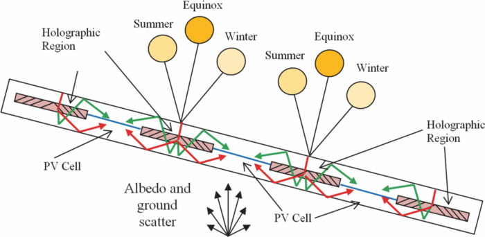 The overall holographic concentration achieved by holographic film was found to be stable for the angular variation which occurs naturally with the daily movement of the Sun.7 The seasonal angle variation causes a change in the spectral selectivity of the hologram, causing a change in the diffracted wavelength and a change in the power output of the cell based on the spectral response of the monocrystalline silicon and the available solar spectrum, as seen in Figs. 11 through 13. Fig. 11Comparison of the holographic performance of the generation I and II of Prism Solar Technologies Inc. holographic film for a 7-mm thick test coupon with a 1.2:1 hologram to cell ratio, the values have been normalized to the peak performance of GEN I film. For the equinox condition and a 1:1 ratio, Gen II increases the power output of the cell by 25%. 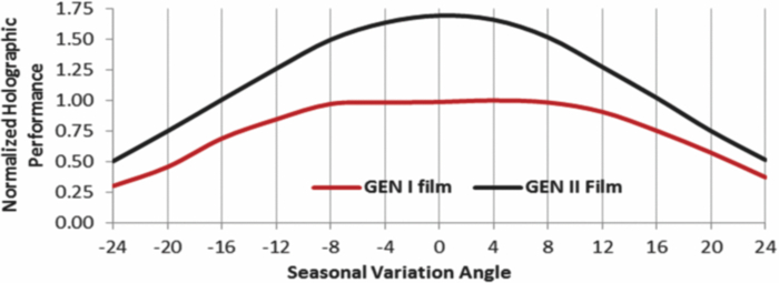 Fig. 13Combined response of the solar spectrum with a modeled response of a crystalline silicon solar cell for AM0 and variations of the AM1.5G standard (Ref. 24). 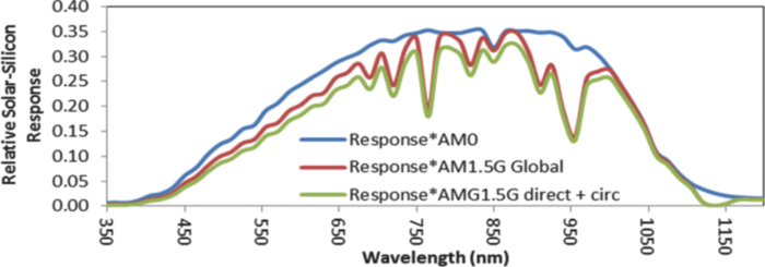 3.Experimental Temperature and Environmental DataTwo holographic and one reference coupon were assembled for the temperature analysis of the HPCs with the same type of diced bifacial solar cells. All of the coupons had the same glass surface area, with dimensions of 304 mm × 406 mm. The reference coupon consisted of nine 125 mm × 25 mm cells, with the cells arranged in three rows of three, spaced 2 mm in either direction. The 1 to 1 coupon consisted of nine 125 mm × 25 mm cells, with the cells arranged in three rows of three, spaced by the holographic film width of 25 mm, and the cell columns separated by 2 mm. The 2 to 1 coupon consisted of fifteen 12.5 mm × 12.5 mm cells, arranged in five rows of three cells, with the cell rows spaced by the holographic film width of 25 mm, and the cell columns separated by 2 mm. The cell/hologram layout for the test coupons as mounted on the white roof on the day of the test is shown in Fig. 2. Fig. 2Experimental setup for the measurement of the cell temperature of the DA holographic panels. The coupons had the following arrangement: (left) 2 to 1 holographic coupon: (middle) packed reference coupon: (right) 1 to 1 holographic coupon. The system was pointed south and tilted for latitude. 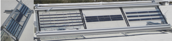 The temperature of the cells was measured with an imbedded thermocouple placed behind the center cell with the test coupons operating under no electrical load condition (open circuit).8, 9 The temperature from each test coupon, along with the global irradiance and wind data is shown in Fig. 3. Fig. 3Experimental temperature data for the HPC coupon modules for a day in late May, 2010. (a) Temperature for the three tested coupons. (b) Wind data for the experiment site (N = 0, E = 90). 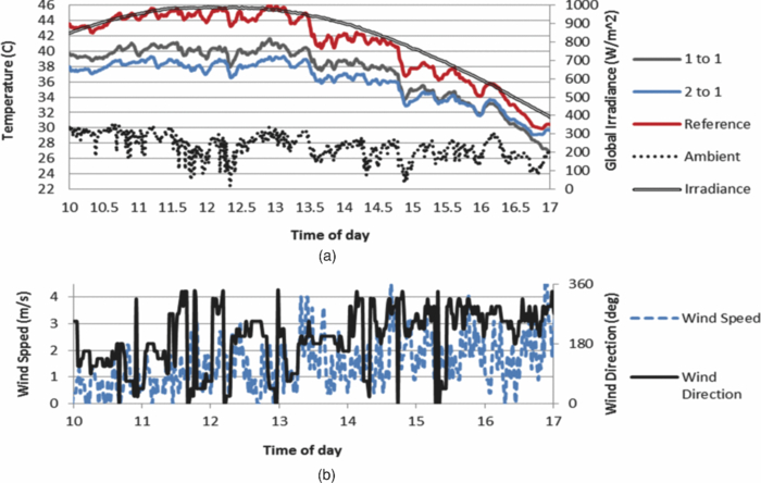 A useful parameter for determining the relationship between the operating cell temperature, the ambient temperature and the irradiance illuminating the module is called the Ross coefficient, and it is given in Eq. 1.8, 9 Using the measured data, the Ross coefficient was calculated for each test coupon. Thus, given certain mounting and environmental conditions, the Ross coefficient can be used to determine the cooling conditions under which a PV panel is operating.8, 9 Table 1 shows common Ross coefficients for different mounting conditions.9 [TeX:] \documentclass[12pt]{minimal}\begin{document}\begin{equation}
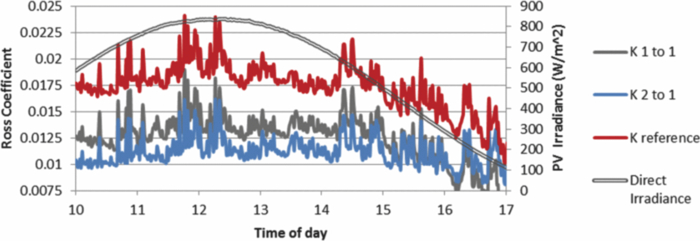
T_{{\rm cell}} = T_{{\rm amb}} + k^\prime\,{ E}_{{\rm PV}},
\end{equation}\end{document} where k′ is the Ross coefficient with units of °Cm2 W−1 or Km2 W−1, EPV flat plate equivalent of the solar irradiance in Wm−2 illuminating the module, Tcell is cell temperature, and Tamb is the ambient temperature. (Tcell − Tamb) has been found to be linear to Ed,10 and its value independent of Tamb (Ref. 8) especially for EPV > 400 Wm−2. Thus, Ross coefficient is directly proportional to the difference between Tcell and Tamb. The smaller (Tcell – Tamb), the lower the drop in cell performance from the negative temperature coefficients for Pmax and Voc. The calculated Ross coefficient for the experimental data as a function of the time of day is shown in Fig. 4. It can be seen that for each test coupon, the calculated Ross parameter stayed relatively stable throughout the testing especially for values of EPV > 400 Wm−2.Table 1Ross coefficients for different mounting conditions for silicon PV panels from Ref. 9.
The cooling effects of the added holographic regions for CIGS cells had already been shown11, 12 and showed a similar measured decrease in the average measured cell temperatures and Ross coefficients. 4.Description of the ModelThe multilayer method for solving heat transfer problems has been successfully applied for planar multilayer structures.13, 14, 15 A simple mathematical model, using the multilayer network approach, was created in C with the use of a specialized, grid-based, heat transfer library called STiMuL.4 The library uses the thermal equivalent circuit for solving the layer problem. From Fourier's heat conduction law, the heat flux for a given direction is given by [TeX:] \documentclass[12pt]{minimal}\begin{document}\begin{equation}
Q = \overrightarrow q \cdot \overrightarrow {u_z } = - k\frac{{dT}}{{dz}},
\end{equation}\end{document}
where k is the material conductivity in Wm−1 K−1, T is the temperature in K, and q is the heat flux in Wm−2. The STiMuL library assumes that all the heat transfered from the stack to the environment occurs in the upper and lowermost surfaces and none in the lateral surfaces. Since the overall lateral area for each test coupon is equal to 9940 mm2 and the total of the upper and lower areas is equal to 246,848 mm2, the assumption that heat transfer to the environment only occurs from those two surfaces is valid. For thin structures, such as the ones modeled here [TeX:] \documentclass[12pt]{minimal}\begin{document}\begin{equation}
h \approx \frac{k}{d},
\end{equation}\end{document} where d is the material thickness.The thermal equivalent resistance, Rthermal, can then be defined as [TeX:] \documentclass[12pt]{minimal}\begin{document}\begin{equation}
R_{{\rm thermal}} = \frac{1}{h} = \frac{d}{k},
\end{equation}\end{document}
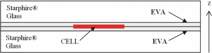
It is useful to treat the thermal resistances as an equivalent electrical circuit.4 A much simplified equivalent circuit is shown in Fig. 5 for a cell embedded in glass with EVA. A diagram to illustrate the simulated structures is shown in Fig. 6. Table 2 shows the actual parameters simulated for each layer in the simulation. Table 2Layer parameters used in the temperature model (Refs. 16, 17, and 18).
Fig. 5Simplified, thermal equivalent circuit diagram of the simulated structure. Heat sources are treated as current sources and temperatures as voltages. The larger the thermal resistances, the more restricted the heat flow will be. 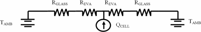 From Table 2, it is clear that the major thermal resistance is that of the glass layers and dominates over all others, limiting the heat transfer from inside the module to the environment. The material conductivity of silicon is larger than 200 Wm−1 K−1 and the cell thickness was ∼200-μm thick. The equivalent thermal resistance of silicon would equal 0.001 × 10⁻³ Km2 W−1. This value is small enough in relation to all the other thermal resistances, that is what was treated as zero for the simulation. For the clear day, see global irradiance data in Fig. 3, the component of the solar radiation (EPV) illuminating the PV panel was approximated as a function of the global irradiance (EG) by [TeX:] \documentclass[12pt]{minimal}\begin{document}\begin{equation}
E_{{\rm PV}} \approx E_{ G} \,\cos ({\rm \theta }_{ s}),
\end{equation}\end{document} where the exact form cos(θs) is given as19
[TeX:] \documentclass[12pt]{minimal}\begin{document}\begin{equation}
\begin{array}{l}
\cos ({\rm \theta }_{ s}) = \sin ({\rm \delta })\cos (\emptyset)\cos ({\rm \beta }) - [{\rm sign}(\emptyset)]\sin ({\rm \delta })\cos (\emptyset)\sin ({\rm \beta })\cos ({\rm \alpha })\\[6pt] \qquad\qquad +\, \cos ({\rm \delta })\cos (\emptyset)\cos ({\rm \beta }) \cos ({\rm \omega }) +
{\rm }[{\rm sign}(\emptyset)]\cos ({\rm \delta })\sin (\emptyset)\sin ({\rm \beta })\cos ({\rm \alpha })\cos ({\rm \omega })\\[6pt]\qquad\qquad +\, \cos ({\rm \delta })\sin ({\rm \alpha })\sin ({\rm \omega })\sin ({\rm \beta }), \\
\end{array}
\end{equation}\end{document} where θs is the angle between the sun's rays and the PV pane, δ is the solar declination angle for the time of the year, ϕ is the latitude of the panel location, β is the slope angle of the panel (usually latitude), α is the Sun azimuth angle, and ω is the true solar time or solar hour. The solar hour is the difference in angle between the selected moment of the day and solar noon. The relationship between the sun, β, θs, α, and the PV panel is shown in Fig. 7. For the case where the PV panel is facing south (α = 0) the previous equation simplifies to19
[TeX:] \documentclass[12pt]{minimal}\begin{document}\begin{equation}
\cos ({\rm \theta }_{ s}) = [{\rm sign}(\emptyset)]\sin ({\rm \delta })\cos (\emptyset)\sin [{\rm abs}(\emptyset) - {\rm \beta]} + \cos ({\rm \delta })\cos [{\rm abs}(\emptyset) - {\rm \beta]}\cos ({\rm \omega }).
\end{equation}\end{document} Fig. 7PV panel layout diagram showing the slope angle β, azimuth angle α, and the Sun's rays incidence angle θs. 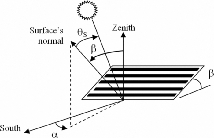 The solar declination angle δ is given by19 [TeX:] \documentclass[12pt]{minimal}\begin{document}\begin{equation}
\delta = 23.45\left\{ {\sin \left[ {\frac{{360\left( {d_n + 284} \right)}}{{365}}} \right]} \right\},
\end{equation}\end{document} where dn is the day number counting from January 1st.The thermal power density EHeat [Wm2] emanating from the cell into the module, and eventually dissipated into the environment, was modeled as [TeX:] \documentclass[12pt]{minimal}\begin{document}\begin{equation}
E_{{\rm Heat}} = E_{{\rm PV}} ( {1 - \rho _g } )( {\tau _g } )( {\overline \alpha _{{\rm PV}} } )\left( {1 + \frac{{\% _{{\rm Holo}} }}{{100}} + \frac{{\% _{{\rm Bi}} }}{{100}}} \right) - \frac{{{\rm IV}_{{\rm dc}} }}{{{\rm AREA}_{{\rm PV}} }},
\end{equation}\end{document}
where ρg is the reflectivity of the glass/air interface taken as 4%. EPV is the flat plate component of the solar radiation hitting the PV panel and is obtained with Eq. 5. [TeX:] $\overline \alpha _{\rm PV}$ is the average absorptivity of the PV cell inside the glass package. Other authors have used values for [TeX:] $\overline \alpha _{\rm PV}$ ranging from 0.90 to 0.94,20, 21 for this work 0.9 was used. τg is transmittance of the glass of the PV package from the manufacturers specifications as 0.9 for the visible and IR18 %Bi is the added power added by the albedo, ground reflected, and scattered components to the back of a bifacial-type PV for those mounting conditions. The bifaciality, that is the light illuminating the back of the coupon relative to the light illuminating the front, was measured at the experiment location at noon and found to be ∼25% for the roof conditions seen in Fig. 2. The roof was coated with a highly reflective white roof coating which helped maximize roof reflected/scattered light contribution to the module. The last term in Eq. 9, IVdc is the product of the dc current and voltages from the system, generally at the maximum power point, divided by the area of the PV generating the power. This provides the electrical power density being generated, going out of the PV system and therefore not being transformed into heat. For the experiment, while operating at the open circuit condition, Idc = 0, the term can be neglected and all the illumination absorbed by the cell is assumed to be transformed into heat which eventually is transferred into the surrounding environment. The %Holo is the added concentration provided by the holograms to PV cells and was taken as 12% for the 1 to 1 hologram/cell ratio and 18% for the 2 to 1 hologram/cell cases, respectively, for the experiment configuration and solar angle declination on the date of the experiment. Since the experiment date a newer, more efficient generation of diffractive film has been developed and its relative performance is seen in Fig. 11. The temperature performance as a function of the holographic contribution was predicted with the developed model, as seen in Fig. 14. Fig. 14Model generated average cell temperatures for the 1 to 1 test coupon configuration (left column) and the 2 to 1 configuration (right column) for various levels of holographic contribution for 800 Wm−2 (top row) and 400 Wm−2 (bottom row) of direct irradiance. The simulated cooling conditions were 15 and 30 Wm−2 and denoted as U15 and U30, respectively. The ambient temperature was assumed to be 30°C. The points where the lines cross is where the average center cell temperature for a holographic type configuration would become hotter than a conventionally arrayed configuration, for the same cooling conditions. 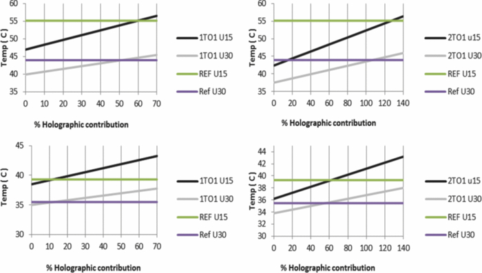 Several assumptions were used while developing the model:
Fig. 12Comparison of the transmission spectra in percentage performance, for normal incidence of the generation I and II of Prism Solar Technologies Inc. holographic film. The increase in diffraction is apparent by the drop of the transmission spectra and the increased bandwidth of Gen II when compared to Gen I.  The overall convective/radiative heat transfer, or the cooling condition, from the top and lower surfaces of glass used in the modeling were 15, 20, 25, and 30 Wm−2. These values are based on the expected convection heat transfer and temperature gradients at the glass layers. Using formulas and results summarized8, 20 for convection heat exchange for winds at 1 m/s, the heat transfer can vary significantly, from about 1.2 Wm−2 K−1 up to 17.1 Wm−2 K−1 for various wind directions. For these wind conditions, the forced convection caused by the movement of air over the panel dominates over all other heat transfer mechanisms.8 The average wind speed for the experiment site was larger than 1 m/s, assuring that convection dominated. 5.Validation of the ModelA series of heat maps, at the solar cell layer, was generated for each of the previously stated cooling condition. In Fig. 8, the heat maps are presented for the lowest and highest cooling conditions, 15 and 30 Wm−2, respectively, for an illumination level of 800 Wm−2 for each of the test coupon configurations. From these heat maps, the average cell temperature for the centermost cell of the arrays was found and subtracted from the simulated ambient temperature of 30C. These results are shown in Fig. 9 against the measured experimental data. The Ross coefficients simulated for the different cooling conditions were also calculated from the slope of Fig. 9 and compared to the Ross coefficients calculated from the measured data. The resulting plots are shown in Fig. 10. Fig. 8Model generated heat maps at the solar cell layer for an EPV of 800 Wm−2 and a heat transfer of 15 Wm−2 (a) and 30 Wm−2 (b) for the glass surfaces for the test coupon configurations. The leftmost figures show the heat maps for the reference coupon, the middle ones for the 1 to 1 coupon, and the rightmost ones for the 2 to 1 test coupons. The color scales vary from 30°C (low end) to 56°C (high end). 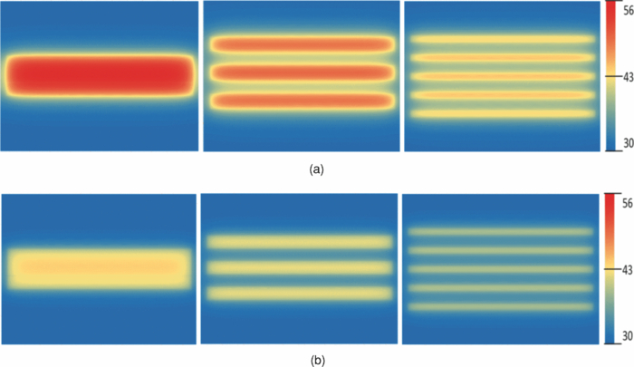 Fig. 9(a) The reference coupon, (b) the 1 to 1 reference coupon, and (c) the 2 to 1 test coupon model generated average cell temperatures difference (Tcell−Tamb) for the centermost cells in test arrays for various levels of irradiance and under various cooling conditions. The models are compared to the experimental data for the solar noon and the afternoon of the experiment date. The model assumed a constant ambient temperature of 30°C. The simulated cooling conditions were 15, 20, 25, and 30 Wm−2 and denoted as U15, U20, U25, and U30, respectively. 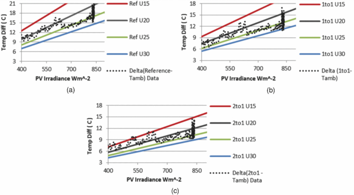 Fig. 10(a) The reference coupon, (b) the 1 to 1 reference coupon, and (c) the 2 to 1 test coupon model generated Ross coefficients [Km2 W−1] for various levels of direct irradiance under various cooling conditions. The models are compared to the experimental data for the solar noon and the afternoon of the experiment date. The model assumed a constant ambient temperature of 30°C. The simulated cooling conditions were 15, 20, 25, and 30 Wm−2 and denoted as U15, U20, U25, and U30, respectively. 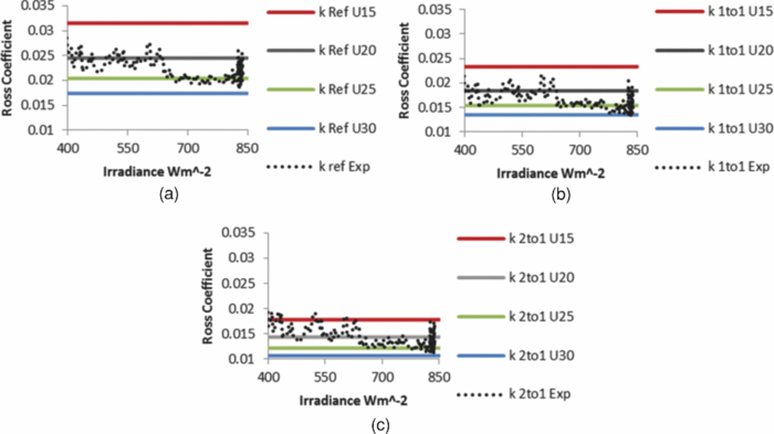 Figures 9 and 10 show a change in the measured temperature and the calculated Ross coefficients at ∼600 Wm−2, corresponding to a shift in the average wind direction at that illumination for the measured data, as shown in Fig. 3. From Fig. 9, the cooling conditions were shown to match 20 to 30 Wm−2 and from Fig. 10, it can be seen that the Ross coefficient indicates that the larger the hologram to cell ratio, the larger the cooling effect upon the PV cell. 6.Holographic Film ImprovementA newer, second generation of holographic film was developed after the experiment was carried out, which has yielded a significant holographic performance increase when compared to the first generation, both in peak, spectral bandwidth, and season angular performance, as seen in Figs. 11 and 12. Figure 13 shows the combined response of crystalline silicon with several standard air mass conditions. A comparison of Figs. 12 and 13 illustrates that the peak of the dip in the transmission spectra of the holograms matches the peak of the combined silicon/air mass response. With the added photons provided by the improved holographic film, the cell temperature is expected to increase. The modeled temperature difference for the 1 to 1 holographic case was simulated for 400 and 800 W/m^2 of incoming irradiance, as a function of the holographic contribution of the holograms, keeping the bifaciality and other parameter constant in Eq. 9. The results are shown in Fig. 14. 7.Temperature Effects on the Output PowerThe temperature coefficient at Pmax, in percentage, of a PV module is defined as [TeX:] \documentclass[12pt]{minimal}\begin{document}\begin{equation}
TC_{P{\rm Max}} (\%) = \frac{{\frac{{dP_{{\rm mp}} }}{{dT}}}}{{P_{{\rm mp}@25^{\circ} {\rm C}} }}100 = \frac{{\frac{{P_{{\rm mp}@T} - P_{{\rm mp}@25^{\circ} {\rm C}} }}{{T - 25}}}}{{P_{{\rm mp}@ 25^{\circ} {\rm C}} }}100,
\end{equation}\end{document} where Pmp@25°C is the maximum power at 25°C, Pmp@T is the maximum power for a temperature T > 25°C. This coefficient is negative for T > 25°C and for commercial crystalline silicon PV modules it ranges from –0.3%/C22 to –0.5%/C.23, 24For a conventionally packed glass/glass monofacial module, the power from the module normalized for module area is given by [TeX:] \documentclass[12pt]{minimal}\begin{document}\begin{equation}
\frac{{P_{{\rm mono}} }}{{A_{{\rm Module}} }} = \eta E_d \left[ {1 + TC_{P{\rm Max}} \left( {T - 25^\circ {\rm C}} \right)} \right].
\end{equation}\end{document}
For a conventionally packed glass/glass bifacial module, the power from the module, normalized for module area is given by [TeX:] \documentclass[12pt]{minimal}\begin{document}\begin{equation}
\frac{{P_{{\rm Bi}} }}{{A_{{\rm Module}} }} = \eta E_d \left( {1 + \frac{{\% _{{\rm Bi}} }}{{100}}} \right)\left[ {1 + TC_{P{\rm Max}} \left( {T - 25^\circ {\rm C}} \right)} \right].
\end{equation}\end{document}
For a dual aperture HPC module the power from the module, normalized for module area is given by [TeX:] \documentclass[12pt]{minimal}\begin{document}\begin{eqnarray}
\frac{{P_{{\rm HPC}} }}{{A_{{\rm Module}} }} = \eta E_d \left[ {\frac{{A_{{\rm PV}} }}{{A_{{\rm Module}} }}\left( {1 + \frac{{\% _{{\rm Bi}} }}{{100}}} \right) + \frac{{A_{{\rm Holo}} }}{{A_{{\rm Module}} }}\left( {\frac{{\% _{{\rm Holo}} }}{{100}}} \right)} \right]\left[ {1 + TC_{P{\rm Max}} \left( {T - {25^\circ}{\rm C}} \right)} \right], \nonumber\\
\end{eqnarray}\end{document} where η is the PV cell efficiency, APV is the photovoltaic area, AHolo is the holographic area, and AModule is the area of the module for the front aperture. All the other variables have been previously defined.Assuming %Bi = 25, APV/AModule = 0.50, AHolo/AModule = 0.50, the same PV cell efficiency, same illumination, and roof conditions as the test at Prism Solar Technologies Tucson, normalized to the Pmono case. The relative powers from each type of module are redefined as P′Mono, P′Bi, P′HPC. Table 3 shows the relative power for different cell temperature coefficients; the higher the cell temperature coefficient, the higher the resulting relative power. Table 3Relative power outputs with and without temperature effects for a monofacial, bifacial, and a 1 to 1 HPC module. Glass-glass construction was assumed as well as even illumination and absorption in the back of all the cases. The holographic contributions were 12% to match the Gen I at the test date and 25% for the peak of Gen II holographic contribution.
8.ConclusionsThe temperature effects on the PV cells, by having 1 to1 and 2 to 1 holographic versus silicon bifacial regions was presented with measured data and compared to a theoretical model. The larger the extended glass regions, in relation to the silicon regions, the lower the resulting average cell temperature in both the experimental and simulated conditions. The model and experimental data matched when comparing the Ross coefficients, which includes the effect of the direct irradiance, for the range of cooling conditions simulated in this work and observed during the experiment. Both sets of data show that as the holographic regions increased in relation to the silicon area, the Ross coefficient decreased, indicating that the silicon cells in the spaced array were dissipating heat into the environment faster than the conventionally packed coupons, for the same environment and mounting conditions. The measured data and the model developed suggests that the cooling effect is more pronounced under poor cooling and high irradiance conditions when comparing a test coupon with extended regions to a conventionally packed PV coupon. The improved operating temperature of the cell will improve the cell operating efficiency when compared to a conventionally assembled test coupon, due to the negative nature of the Pmax temperature coefficient for silicon crystalline cells. This improvement is dependent on the light hitting the back of the module and the concentration provided by the holographic film, the higher these are, the lower the improvement. Depending on the temperature coefficient of the cells, holographic performance of the Prism Solar Technologies Inc. film and the cooling conditions under which the PV is operating, the relative improvements in maximum power output should be in the 0.7% to 3.3% range at the 800 Wm−2 illumination levels when compared to a comparably built standard packed module. AcknowledgmentsThis material is based in part upon work supported by the National Science Foundation (NSF) under Grant Nos. 0912797 and 0925085 and by the Science Foundation Arizona Grant No. 3443831. Any opinions, findings, and conclusions or recommendations expressed in this material are those of the author(s) and do not necessarily reflect the views of the National Science Foundation. ReferencesR. K. Kostuk, J. Castillo, J. M. Russo, and G. Rosenberg,
“Spectral-shifting and holographic planar concentrators for use with photovoltaic solar cells,”
Proc. SPIE, 6649 66490I
(2007). http://dx.doi.org/10.1117/12.736542 Google Scholar
R. Kostuk and G. Rosenberg,
“Analysis and design of holographic solar concentrators,”
Proc. SPIE, 7043 70430I
(2008). http://dx.doi.org/10.1117/12.793895 Google Scholar
R. K. Kostuk, J. M. Castro, and D. Zhang,
“Energy collection efficiency of low concentration holographic planar concentrators,”
Proc. SPIE, 7769 776902
(2010). http://dx.doi.org/10.1117/12.859713 Google Scholar
J. Russo, J. Castillo Aguilella, and G. Rosenberg,
“Dual aperture holographic planar concentrator photovoltaic module energy harvesting performance,”
OSA Technical Digest,
(2010). Google Scholar
J. M. Russo, J. E. Castillo, E. Aspnes, and G. Rosenberg,
“Seasonal and low light performance of a dual aperture holographic planar concentrator photovoltaic module,”
OSA Technical Digest,
(2010). Google Scholar
J. E. Castillo, J. M. Russo, E. Aspnes, and G. Rosenberg,
“Low concentration planar holographic cigs,”
OSA Technical Digest,
(2010). Google Scholar
E. Skoplaki, A. G. Boudouvis, and J. A. Palyvos,
“A simple correlation for the operating temperature of photovoltaic modules of arbitrary mounting,”
Sol. Energy Materi. Sol. Cells, 92 1393
–1402
(2008). http://dx.doi.org/10.1016/j.solmat.2008.05.016 Google Scholar
E. Skoplaki and J. A. Palyvos,
“Operating temperature of photovoltaic modules: A survey of pertinent correlations,”
Renewable Energy, 34
(1), 23
–29
(2009). http://dx.doi.org/10.1016/j.renene.2008.04.009 Google Scholar
J. W. Stultz,
“Thermal and other tests of photovoltaic modules performed in natural sunlight,”
(1978). Google Scholar
J. Castillo, J. Russo, D. Zhang, R. Kostuk, and G. Rosenberg,
“Low holographic concentration effects on CIGS,”
Proc. SPIE, 7769 77690L
(2010). http://dx.doi.org/10.1117/12.862038 Google Scholar
J. Castillo, J. Russo, S. Herr-Cardillo, R. Kumar, and G. Rosenberg,
“Reduced temperature of holographic planar concentrators,”
OSA Technical Digest,
(2010). Google Scholar
D. H. Chien, C. Y. Wang, and C. C. Lee,
“Temperature solution of five-layer structure with an embedded circular source,”
177
–182
(1992). Google Scholar
A. G. Kokkas,
“Thermal analysis of multiple-layer structures,”
IEEE Trans. Electron Devices, ED-21
(11), 674
–681
(1974). http://dx.doi.org/10.1109/T-ED.1974.17993 Google Scholar
J. Albers,
“An exact recursion relation solution for the steady-state surface temperature of a general multilayer structure,”
IEEE Trans. Compon. Packag. Manuf. Technol., 18
(1), 31
–38
(1995). http://dx.doi.org/10.1109/95.370732 Google Scholar
B. Lee, J. Z. Liu, B. Sun, C. Y. Shen, and G. C. Dai,
“Thermally conductive and electrically insulating EVA composite encapsulants for solar photovoltaic (PV) cell,”
eXPRESS Polymer Letters, 2
(5), 357
–363
(2008). http://dx.doi.org/10.3144/expresspolymlett.2008.42 Google Scholar
S. Ghose, K. A. Watson, D. C. Working, J. W. Connell, J. G., Smith Jr., and Y. P. Sun,
“Thermal conductivity of ethylene vinyl acetate copolymer/nanofiller blends,”
Compos. Sci. Technol., 68
(7–8), 1843
–1853
(2008). http://dx.doi.org/10.1016/j.compscitech.2008.01.016 Google Scholar
A. Luque and S. Hegedus, Handbook of Photovoltaic Science and Engineering, John Wiley & Sons, West Sussex, England
(2003). Google Scholar
G. Notton, C. Cristofari, M. Mattei, and P. Poggi,
“Modelling of a double-glass photovoltaic module using finite differences,”
Appl. Therm. Eng., 25
(17–18), 2854
–2877
(2005). http://dx.doi.org/10.1016/j.applthermaleng.2005.02.008 Google Scholar
A. A. Hegazy,
“Comparative study of the performances of four photovoltaic/thermal solar air collectors,”
Energy Convers. Manage., 41 861
–881
(1999). http://dx.doi.org/10.1016/S0196-8904(99)00136-3 Google Scholar
|