One-axis tracking holographic planar concentrator systems

Deming Zhang; Jose M. Castro; Raymond K. Kostuk

doi:10.1117/1.3590943

1 January 2011 One-axis tracking holographic planar concentrator systems

Deming Zhang, Jose M. Castro, Raymond K. Kostuk

Author Affiliations +

Journal of Photonics for Energy, Vol. 1, Issue 1, 015505 (January 2011). https://doi.org/10.1117/1.3590943

Abstract

A design methodology for low-concentration ratio holographic solar concentrators with one-axis tracking is investigated. This methodology maximizes the energy collected by cascaded holographic gratings and reduces diffracted beam cross talk between gratings. Several types of transmission gratings, optimized to work with single-axis tracking systems, are used in a cascaded configuration to concentrate a large fraction of the useable solar spectrum on the surface of photovoltaic cells. A model is developed that determines the energy yield of the holographic planar concentrator (HPC). Good agreement is found between simulation and measurement of a prototype system. Simulation of an optimized HPC design shows that 80% optical efficiency at 2X geometric concentration ratio is possible. The acceptance angle in the nontracking direction is ±65 deg, and a ±16-deg tracking tolerance is sufficient to maintain 80% of the maximum optical efficiency. Simulation also shows that the single-axis tracking HPC system has a 43.8% increase in energy yield compared to a nontracking holographic solar concentrator.

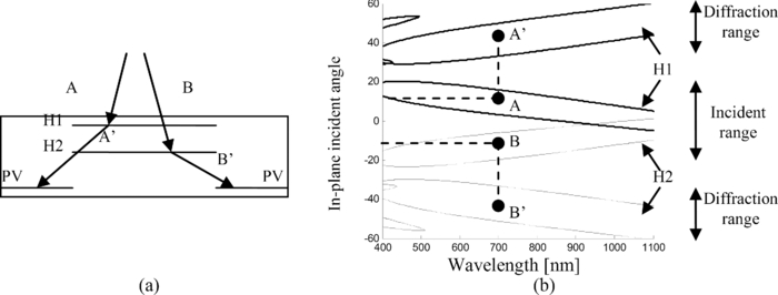
1. Introduction

Currently, a great deal of effort is being placed on flat-panel modules that are fully populated with photovoltaic (PV) cells and also on high-concentration ratio systems with 100–1000X concentration ratios. Flat-panel modules can accept light over a 180-deg acceptance angle and are typically used at a fixed angle relative to the position of the sun. However, it has been shown that the energy yield of flat-panel systems can be improved by a significant factor (15–40%) with single-axis tracking.^{1, 2, 3, 4} This becomes beneficial especially for higher cost high-efficiency crystalline silicon cells. High-concentration photovoltaic (CPV) systems require two-axis tracking because of the relatively narrow acceptance angle dictated by the brightness theorem or power conservation principles.⁵ The higher cost of the tracking system can be offset by the higher power that can be extracted from multijunction PV cells.

Another operating domain is low (2X) to medium (50X) concentration ratio concentrator systems. There are several motivations for this group of systems. First, higher output power and energy yields are possible from the same area because higher efficiency cells can be used. This is an important consideration when deployment areas are limited, as in residential and commercial rooftop applications. The cost of the system can be lower than conventional flat-panel systems by minimizing the use of expensive PV converters. Finally, the tracking and PV cell cooling requirements are less complex than high-concentration ratio systems that can potentially provide system cost and reliability benefits.

Holographic optical elements (HOEs) have been proposed for a variety of solar collection applications^{5, 6, 7, 8} are well suited for low concentration ratio PV systems. High diffraction efficiency HOEs can be inexpensively fabricated on large-area glass or polymer substrates.⁶ This manufacturing technology has been used to fabricate on-axis transmission holographic lenses for solar concentration⁶ and nontracking holographic planar concentrator (HPC) holographic elements.^{7, 8, 9} HOEs can achieve very high diffraction efficiency in layers that are a few microns thick. This characteristic allows incident rays to be deflected at very large angles and a reduction in the height of the concentrator.

Another advantage of HPCs that has recently been reported is that they have better cooling properties than fully PV-populated flat-panel modules.⁹ Previous studies for passive tracking HPC systems have shown that up to 47% of incident annual solar energy illuminating the hologram surface can be diffracted to the PV cell surface.⁸ This results in a module optical system efficiency of 70% with a 1:1 hologram-to-PV-area ratio. HPC used in combination with a tracking system allows more freedom in the design of the hologram. However, the performance of HPC with one-axis tracking has not been analyzed.

In this paper, a methodology to design tracking holographic solar concentrators for low-concentration ratio systems is investigated. This methodology focuses on maximizing the energy collected by each holographic grating and reducing the cross-coupling effects between holograms. Cascaded transmission grating configurations are optimized for use with single-axis tracking systems. The energy yield of the tracking HPC is analyzed and compared to modules that are fully populated with PV cells. The simulation and experimental results indicate that 80% optical efficiency is possible compared to 70% for a nontracking HPC system.

2. Holographic Planar Concentrator System Overview

The basic HPC system is illustrated in Fig. 1. Concentration is achieved by diffracting incident sunlight onto nearby PV cells. Transmission holograms are designed to provide the required diffraction. The diffracted light can reach the PV cell directly or after total internal reflection (TIR) at the substrate-air interface.

Fig. 1

Component layout of an HPC. The z-axis is normal to the hologram surface, and the fringes of the grating are parallel to the x-axis.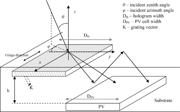

The performance of the HPC is evaluated with respect to acceptance angle, geometric concentration ratio, optical efficiency, and energy collection efficiency as will be described in Sec. 3. Critical parameters to optimize the performance of the HPC include the hologram's Bragg angles, peak diffraction efficiency (DE), and the spectral and angular bandwidth that is diffracted.^{8, 10} The three-dimensional layout in Fig. 1 is used to show two cases of light diffraction useful for the HPC design.

For incident light in the yz plane (φ = 0 deg, –90 < θ < 90 deg), the wavelength for peak diffraction efficiency is highly dependent on the incident angle.^{8, 10, 11} This effect reduces the acceptance angle of the HPC in the yz plane. For light with incident vectors in the xz plane (φ = 0 deg, –90 < θ < 90 deg), the change of peak wavelength is much less dependent on the incident angle. Therefore, the acceptance angle of the HPC in the xz plane is much larger than in the yz direction. In this paper, the φ = 0 deg direction defines the in-plane direction, and φ = 90 deg direction specifies the out-of-plane direction. These directions will be aligned with the sun's daily and seasonal movements for optimal energy collection.

The diffracted spectrum of the hologram can be customized for different bandgap PV materials, such as silicon, GaAs, CIGS, and CdTe. However, the typical spectral bandwidth of a single hologram (<300 nm FWHM) is not sufficient to collect the available energy in the solar spectrum. In the case of silicon solar cells, which utilize solar radiation between 400 and 1100 nm wavelength, at least two holograms are required to capture a significant amount of the energy in this spectral range. There are limitations in using more than two holograms in a stack,⁸ which are reviewed in Sec. 4.

It has been previously shown that for a static HPC with two cascaded holograms, 47% of the usable incident solar energy can be diffracted and collected by the PV cell.⁸ However, it is difficult to achieve full-spectrum concentration and still maintain coverage over the large range of solar incident angles.

By following the large daily movement of the sun, a single-axis tracking system significantly changes the design and increases the energy yield of the PV system. Because holograms are more sensitive to in-plane incident angle changes, tracking in this direction can significantly improve performance. Tracking is not necessary in the out-of-plane direction because the diffraction efficiency of the grating has a much broader angular acceptance range. Using this single-axis tracking configuration, there are more degrees of freedom in optimizing collection of the solar spectrum with minimal cross talk between gratings, as shown in Sec. 4.

3. System Analysis

The basic algorithm to determine the solar illumination reaching the surface of the PV cell in an HPC module and converted into electrical power consists of the following:

1. performing a ray trace through the hologram aperture and optical substrate
2. computing Fresnel losses at the optical interfaces
3. computing the diffraction efficiency of the ray at the particular angle of incidence and wavelength and weight the ray with this value
4. integrating the weighted ray efficiencies for all rays that intercept the PV cell surface for the combined air mass and PV cell responsivity spectrum

The integrated weighted ray efficiency is then normalized to the integrated available solar energy without optical loss. This parameter provides an estimate of the efficiency of the holographic collection system. A detailed description of this process was presented in Ref. 8. A summary of the main elements of this model are provided in Secs. 3.1, 3.2, 3.3, 3.4, 3.5.

3.1.

Diffraction Efficiency Model

The diffraction efficiency of the holographic grating is calculated with Kogelnik's coupled wave theory.¹¹ The coupled wave theory is an analytical method that gives close approximation to experimental results.⁸

At wavelength λ, the grating vector K is

[TeX:] \documentclass[12pt]{minimal}\begin{document}\begin{equation} \vec K = \left[ {\begin{array}{*{20}c} {K_x } \\[5pt] {K_y } \\[5pt] {K_z } \\[5pt] \end{array}} \right] = \frac{{2\pi n}}{\lambda }\left[ {\begin{array}{*{20}c} {\sin \theta _{\rm c} \sin \varphi _{\rm c} - \sin \theta _{{\rm ref}} \sin \varphi _{{\rm ref}} } \\[5pt] {\sin \theta _{\rm c} \cos \varphi _{\rm c} - \sin \theta _{{\rm ref}} \cos \varphi _{{\rm ref}} } \\[5pt] {\cos \theta _{\rm c} - \cos \theta _{{\rm ref}} } \\[5pt] \end{array}} \right], \end{equation}\end{document}

\vec{K} = [\begin{matrix} K_{x} \\ K_{y} \\ K_{z} \end{matrix}] = \frac{2 π n}{λ} [\begin{matrix} \sin θ_{c} \sin ϕ_{c} - \sin θ_{ref} \sin ϕ_{ref} \\ \sin θ_{c} \cos ϕ_{c} - \sin θ_{ref} \cos ϕ_{ref} \\ \cos θ_{c} - \cos θ_{ref} \end{matrix}],

where θ_c and θ_ref are construction and reference beam zenith angles in the grating medium, φ_c and φ_ref are construction and reference beam azimuth angles in the grating medium relative to the grating surface normal, and n is the mean refractive index of the grating medium.

For an incident beam with propagation vector,

[TeX:] \documentclass[12pt]{minimal}\begin{document}\begin{equation} \vec \rho = \beta \left[ \begin{array}{l} \begin{array}{*{20}c} {\sin \theta } & {\sin \varphi } \\ {\sin \theta } & {\cos \varphi } \\ \end{array} \\ \,\,\,\,\,\,\cos \theta \\ \end{array} \right],\,\,\,\,\,\beta = \frac{{2\pi n}}{\lambda }, \end{equation}\end{document}

\vec{ρ} = β [\begin{matrix} \begin{matrix} \sin θ & \sin ϕ \\ \sin θ & \cos ϕ \end{matrix} \\ \cos θ \end{matrix}], β = \frac{2 π n}{λ},

with λ being the incident wavelength, and θ and φ are the incident zenith angle and azimuth angle, respectively. The corresponding diffraction efficiency is given by

[TeX:] \documentclass[12pt]{minimal}\begin{document}\begin{equation} \eta = \frac{{\sin ^2 (\nu ^2 + \xi ^2)^{1/2} }}{{1 + \xi ^2 /\nu ^2 }}, \end{equation}\end{document}

η = \frac{\sin^{2} {(ν^{2} + ξ^{2})}^{1 / 2}}{1 + ξ^{2} / ν^{2}},

where

[TeX:] \documentclass[12pt]{minimal}\begin{document}\begin{equation*} \nu = \frac{{\pi n_1 d}}{{\lambda (c_{\rm R} c_{\rm S})^{1/2} }},\,\,\,\xi = \frac{{\vartheta d}}{{2c_{\rm S} }},\,\,\,\vartheta = \frac{{\beta ^2 - \left| \sigma \right|^2 }}{{2\beta }},\,\,\,\vec \sigma = \vec \rho - \vec K. \end{equation*}\end{document}

ν = \frac{π n_{1} d}{λ {(c_{R} c_{S})}^{1 / 2}}, ξ = \frac{ϑ d}{2 c_{S}}, ϑ = \frac{β^{2} - {|σ|}^{2}}{2 β}, \vec{σ} = \vec{ρ} - \vec{K} .

For nontracking HPC systems, the fringe direction (Fig. 1) is aligned along the east-west direction for better daily energy collection. For a single-axis tracking HPC system, the fringe direction is aligned in a north-south direction because the HPC surface is tracked toward the east-west movement of the sun during the day.

3.2.

Optical System Model

The geometric concentration ratio of the system is given by

[TeX:] \documentclass[12pt]{minimal}\begin{document}\begin{equation} C = \frac{{A_{\rm o} }}{{A_{{\rm PV}} }} = \frac{{D_{\rm H} + D_{{\rm PV}} }}{{D_{{\rm PV}} }}, \end{equation}\end{document}

C = \frac{A_{o}}{A_{PV}} = \frac{D_{H} + D_{PV}}{D_{PV}},

where A_o and A_PV are respectively the area of the concentrator and PV receiver in the unit cell (Fig. 1). D_H is the width of hologram and D_PV is the width of the PV cell.

Power generation from direct illumination on the PV cell at time t on day number d_n is given by

[TeX:] \documentclass[12pt]{minimal}\begin{document}\begin{equation} P_{{\rm PV}} (t,d_n) = F_{o - e} A_{{\rm PV}} \cos [\theta (t,d_n),\varphi (t,d_n)]T[\theta (t,d_n),\varphi (t,d_n)] \int\nolimits_\lambda {{\rm SR}(\lambda)E_{{\rm AM15D}} (\lambda)d\lambda },\end{equation}\end{document}

P_{PV} (t, d_{n}) = F_{o - e} A_{PV} \cos [θ (t, d_{n}), ϕ (t, d_{n})] T [θ (t, d_{n}), ϕ (t, d_{n})] \int_{λ} SR (λ) E_{AM 15 D} (λ) d λ,

where θ(t, d_n) and φ(t, d_n) are the incident zenith and azimuth angles in air as a function of time of day t and day number d_n. T is the transmission of substrate-air interfaces for randomly polarized light, A_PV is the PV cell area, SR is the spectral responsivity of a particular PV cell [Fig. 2], E_AM15D is the direct and circumsolar component of the solar irradiance incident on the PV cell surface [Fig. 2]. The parameter F_o-e = FF – V_oc, with FF as the fill factor and V_oc as the open-circuit voltage. The fill factor is defined as FF = P_max/I_scV_oc. P_max is the maximum electrical power operating point and I_sc is the short-circuit current.

Fig. 2

(a) The spectral responsivity of a silicon solar cell and (b) AM 1.5 direct and circumsolar spectral irradiance.

Power generated by light diffracted from a hologram adjacent to a PV cell and intercepting the surface of the cell at time t on day number d_n is calculated by

[TeX:] \documentclass[12pt]{minimal}\begin{document}\begin{eqnarray} P_{\rm H} (t,d_n) &=& F_{{\rm o} - e} A_{\rm H} \cos [\theta (t,d_n),\varphi (t,d_n)]T[\theta (t,d_n),\varphi (t,d_n)]\nonumber\\ && \times \int\nolimits_\lambda {DE[\lambda,\theta '(t,d_n),\varphi '(t,d_n)]SR(\lambda)E_{{\rm AM15D}} (\lambda)d\lambda }, \end{eqnarray}\end{document}

\begin{matrix} P_{H} (t, d_{n}) & = & F_{o - e} A_{H} \cos [θ (t, d_{n}), ϕ (t, d_{n})] T [θ (t, d_{n}), ϕ (t, d_{n})] \\ \times \int_{λ} D E [λ, θ^{'} (t, d_{n}), ϕ^{'} (t, d_{n})] S R (λ) E_{AM 15 D} (λ) d λ, \end{matrix}

where θ^′(t, d_n) and φ^′(t, d_n) are the incident zenith and azimuth angles in the grating medium, A_H is the hologram area, and DE is the spectral and angular-dependent diffraction efficiency.

The power concentration factor (PCF) is defined as follows:

[TeX:] \documentclass[12pt]{minimal}\begin{document}\begin{equation} {\rm PCF}(t,d_n) = \frac{{P_{{\rm PV}} (t,d_n) + P_{\rm H} (t,d_n)}}{{P_{{\rm PV}} (t,d_n)}}, \end{equation}\end{document}

PCF (t, d_{n}) = \frac{P_{PV} (t, d_{n}) + P_{H} (t, d_{n})}{P_{PV} (t, d_{n})},

the optical efficiency is

[TeX:] \documentclass[12pt]{minimal}\begin{document}\begin{equation} \eta _{\rm o} (t,d_n) = T[\theta (t,d_n),\varphi (t,d_n)]\frac{{{\rm PCF}(t,d_n)}}{C}.\end{equation}\end{document}

η_{o} (t, d_{n}) = T [θ (t, d_{n}), ϕ (t, d_{n})] \frac{PCF (t, d_{n})}{C} .

The optical concentration ratio on the PV cell is calculated with

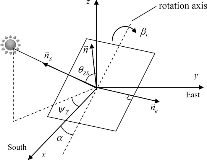
[TeX:] \documentclass[12pt]{minimal}\begin{document}\begin{equation} C_{\rm o} (t,d_n) = C \cdot \eta _{\rm o} (t,d_n) = T[\theta (t,d_n),\varphi (t,d_n)][{\rm PCF}(t,d_n)]. \end{equation}\end{document}

C_{o} (t, d_{n}) = C \cdot η_{o} (t, d_{n}) = T [θ (t, d_{n}), ϕ (t, d_{n})] [PCF (t, d_{n})] .

The acceptance angle of the concentrator is defined as the angle at which the optical efficiency η_o(θ,φ) drops to 90% of the maximum value. The acceptance angle of the HPC module is asymmetric and will be shown to have a much larger out-of-plane acceptance angle than in-plane angular range.

The ray-trace portion of the model is performed using the nonsequential feature of the ZEMAX simulation program. This allows both the angle of incidence and the spectrum to be varied as required for solar illumination. Kogelnik's coupled wave calculation for the diffraction efficiency is computed for each incident ray angle and wavelength through a dynamic link library file coupled to the ZEMAX ray trace.

3.3.

Solar Illumination Modeling

The solar declination angle δ is a function of day number d_n, and in our model is assumed to remain constant over the course of a day,

[TeX:] \documentclass[12pt]{minimal}\begin{document}\begin{equation} \delta \approx 23.45\deg \,\,\sin \left[ {\frac{{2\pi (d_n + 284)}}{{365}}} \right]. \end{equation}\end{document}

δ \approx 23.45 \deg \sin [\frac{2 π (d_{n} + 284)}{365}] .

The solar zenith angle θ_ZS and azimuth angle ψ_Z (Fig. 3) are functions of the declination angle and are given by¹²

[TeX:] \documentclass[12pt]{minimal}\begin{document}\begin{equation} \theta _{{\rm ZS}} = \cos ^{ - 1} (\sin \delta \,\,\sin \phi + \cos \delta \,\,\cos \phi \,\,\cos \omega), \end{equation}\end{document}

θ_{ZS} = \cos^{- 1} (\sin δ \sin φ + \cos δ \cos φ \cos ω),

[TeX:] \documentclass[12pt]{minimal}\begin{document}\begin{equation} \psi _{\rm Z} = \cos ^{ - 1} \left[ {{\rm sign}(\phi)\frac{{\cos \theta \,\,\sin \phi - \sin \delta }}{{\sin \theta \,\,\cos \phi }}} \right], \end{equation}\end{document}

ψ_{Z} = \cos^{- 1} [sign (φ) \frac{\cos θ \sin φ - \sin δ}{\sin θ \cos φ}],

where ϕ is the geographic latitude, positive for north hemisphere and negative for south hemisphere, ω is the true solar time,

[TeX:] \documentclass[12pt]{minimal}\begin{document}\begin{equation} \omega = 15 \times (t - AO - 12) - ({\rm LL} - {\rm LH}) \end{equation}\end{document}

ω = 15 \times (t - A O - 12) - (LL - LH)

in which t is the local standard time, AO is the local time difference relative to the start of the local time zone, LL is the local longitude, and LH is the local reference longitude with respect to the Greenwich Meridian.

Fig. 3

Angle conventions for the sun's zenith angle and azimuth angle relative to a horizontal surface (xy plane). The one-axis tracker rotates around an axis tilted at α in the N-S direction.

An ideal one-axis tracking system maintains the optimum angle towards the sun by rotating around a north-south axis tilted at an angle α. The angle β_t is defined as the tracker rotation angle relative to the tracker position at solar noon,

[TeX:] \documentclass[12pt]{minimal}\begin{document}\begin{equation} \beta _{\rm t} = \tan ^{ - 1} \left( {\frac{{\sin \theta _{{\rm ZS}} \sin \psi _{\rm Z} }}{{\sin \alpha \,\,\sin \theta _{{\rm ZS}} \cos \psi _{\rm Z} + \cos \alpha \,\,\cos \theta _{{\rm ZS}} }}} \right),\quad - 90 < {\rm \beta }_{\rm t} < 90\,\,\deg. \end{equation}\end{document}

β_{t} = \tan^{- 1} (\frac{\sin θ_{ZS} \sin ψ_{Z}}{\sin α \sin θ_{ZS} \cos ψ_{Z} + \cos α \cos θ_{ZS}}), - 90 < β_{t} < 90 \deg .

The tracking axis tilt angle α is selected to be equal to the latitude angle for polar one-axis tracking, and zero for horizontal N-S one-axis tracking.

The direct normal irradiance E_DNI received by a surface perpendicular to a ray directly from the sun is estimated by¹³

[TeX:] \documentclass[12pt]{minimal}\begin{document}\begin{equation} E_{{\rm DNI}} = 1.367 \times 0.7^{{\rm AM}^{0.678} }, \end{equation}\end{document}

E_{DNI} = 1.367 \times 0 . 7^{{AM}^{0.678}},

where the air mass is AM = 1/cos θ_ZS.

Ideal dual-axis trackers can constantly maintain the panel surface orthogonal to direct rays from the sun. The single-axis tracking panel lacks one degree of freedom and does not receive the full E_DNI value. The irradiance received by a panel with single-axis tracking is reduced to a value of

[TeX:] \documentclass[12pt]{minimal}\begin{document}\begin{equation} E = E_{{\rm DNI}} \left[ {\begin{array}{*{20}c} {\sin \theta _{{\rm ZS}} \cos \psi _{\rm Z} } \\[5pt] {\sin \theta _{{\rm ZS}} \sin \psi _{\rm Z} } \\[5pt] {\cos \theta _{{\rm ZS}} } \\[5pt] \end{array}} \right] \cdot \left[ {\begin{array}{*{20}c} {\cos \beta _t \sin \alpha } \\[5pt] {\sin \beta _t } \\[5pt] {\cos \beta _t \cos \alpha } \\[5pt] \end{array}} \right],\,\,\,\, - 45 < \beta _{\rm t} < 45\,\,\deg. \end{equation}\end{document}

E = E_{DNI} [\begin{matrix} \sin θ_{ZS} \cos ψ_{Z} \\ \sin θ_{ZS} \sin ψ_{Z} \\ \cos θ_{ZS} \end{matrix}] \cdot [\begin{matrix} \cos β_{t} \sin α \\ \sin β_{t} \\ \cos β_{t} \cos α \end{matrix}], - 45 < β_{t} < 45 \deg .

3.4.

Annual Energy Yield Calculation

In Sec. 3.2, the incident zenith angle θ and azimuth angle φ are relative to the module surface normal and hologram fringe orientation (Fig. 1). They can be derived from tracking angle, module tilt angle, and the solar zenith and azimuth angles [see the Appendix, Eqs. 23, 24]. The solar zenith and azimuth angles are functions of time of day t and day number d_n, which can be calculated according to Eqs. 11, 12. The incident zenith angle θ and azimuth angle φ relative to the module surface normal can be expressed as θ(t, d_n) and φ(t, d_n). The corresponding angles θ^′(t, d_n) and φ^′(t, d_n)in the grating medium are calculated with Snell's law.

At a given day with day number d_n, the daily energy yield is

[TeX:] \documentclass[12pt]{minimal}\begin{document}\begin{eqnarray} E_{{\rm day}} (d_n) &=& \int {(P_{\rm H} + P_{{\rm PV}})dt} \nonumber\\ &=& \int\!\! {\int\nolimits_\lambda {F_{{\rm o} - e} D_{\rm f} A_{\rm H} T[\theta (t,d_n),\varphi (t,d_n)]{\rm DE}[\lambda,\theta '(t,d_n),\varphi '(t,d_n)]{\rm SR}(\lambda)E(\lambda,t,d_n)d\lambda } } dt \nonumber\\ && + \int {\int\nolimits_\lambda {F_{{\rm o} - e} D_{\rm f} A_{{\rm PV}} T[\theta (t,d_n),\varphi (t,d_n)]{\rm SR}(\lambda)E(\lambda,t,d_n)d\lambda } } dt, \end{eqnarray}\end{document}

\begin{matrix} E_{day} (d_{n}) & = & \int (P_{H} + P_{PV}) d t \\ = & \int \int_{λ} F_{o - e} D_{f} A_{H} T [θ (t, d_{n}), ϕ (t, d_{n})] DE [λ, θ^{'} (t, d_{n}), ϕ^{'} (t, d_{n})] SR (λ) E (λ, t, d_{n}) d λ d t \\ + \int \int_{λ} F_{o - e} D_{f} A_{PV} T [θ (t, d_{n}), ϕ (t, d_{n})] SR (λ) E (λ, t, d_{n}) d λ d t, \end{matrix}

where E(λ,t,d_n) is the renormalized AM 1.5 spectral irradiance giving an integrated irradiance level calculated according to Eq. 16. The time of day t includes hours with zenith angles θ > 0 deg. D_f is the derating factor considering non-uniform illumination on the PV cell, which is defined as the ratio of fill factors under nonuniform irradiance and uniform irradiance,

[TeX:] \documentclass[12pt]{minimal}\begin{document}\begin{equation} D_{\rm f} = \frac{{{\rm FF}_{{\rm nonuniform}} }}{{{\rm FF}_{{\rm uniform}} }}. \end{equation}\end{document}

D_{f} = \frac{{FF}_{nonuniform}}{{FF}_{uniform}} .

The annual energy yield of the system is obtained by summation of the daily energy yield for 365 days of the year

[TeX:] \documentclass[12pt]{minimal}\begin{document}\begin{equation} E_{{\rm annual}} = \sum\limits_{d_n } {E_{{\rm day}} (d_n)}. \end{equation}\vspace*{-12pt}\end{document}

E_{annual} = \sum_{d_{n}} E_{day} (d_{n}) .

3.5.

Experimental Validation of Optical Simulation

In order to validate the modeling, holograms were fabricated in dichromated gelatin (DCG) with collimated beams with incident angles of 22 and 70 deg in air relative to the hologram surface normal and a construction wavelength of 532 nm. The grating thickness was ∼3 μm, and the effective index modulation was 0.09. The diffraction efficiency was indirectly measured by evaluating the transmittance of the hologram at different angles of incidence. Fresnel reflection losses at the interfaces were also taken into account. The measured diffraction efficiency for this grating is shown in Fig. 4 with the simulated DE in good agreement.

Fig. 4

(a) Simulated (line) and measured (dots) diffraction efficiency as a function of wavelength, at in-plane incident angle θ = 10 deg, φ = 0 deg. (b) The optical efficiency as a function of in-plane incident angle.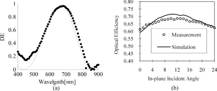

This hologram was used in combination with a silicon PV cell with D_H = D_PV to form an HPC unit cell. An experimental measurement of the optical efficiency of the HPC unit cell was determined by illuminating the combination with an AM 1.5 filtered Xenon arc source and measuring the short-circuit current generated by the PV cell as a function of incident angle. The short-circuit current generated by the HPC unit cell (I_PV + I_H) was divided by the output for an ideal 2X concentrator (i.e., 2I_PV). The result is shown in Fig. 4, which indicates that the optical efficiency for the in-plane angle of incidence remains above 60% over an angular range of 25 deg with a peak optical efficiency near 70%. The peak occurs at the in-plane angle of incidence near 10 deg relative to the hologram normal. The peak corresponds to the best match to the diffracted solar spectrum with the PV cell spectral responsivity and ray overlap on the PV cell surface. The peak is predicted by the simulation, and there is a relatively good agreement over the 0–25 deg incident angle range.

4. Design Criteria and Methodology

Multiple holographic elements are required to diffract incident solar illumination over broad angular and spectral bandwidth. The resulting holographic system must maximize the combined diffraction efficiency of the combination and requires careful consideration of cross-coupling between grating elements. In Secs. 4.1, 4.2, a design methodology for accomplishing these objectives are described and applied to the one-axis tracking HPC system.

4.1.

Holographic System Design

Diffraction efficiency and diffraction angle depend on both the angle and wavelength of incident light. A two-dimensional diffraction efficiency (2-D DE) plot showing the DE as a function of wavelength for different angles of incidence is a helpful tool to verify the effectiveness of a holographic planar concentrator. Figure 5 shows the diffraction efficiency in the yz plane (in plane) as a function of wavelength and in-plane incident angle.

Fig. 5

(a) Single hologram HPC layout and (b) corresponding 2-D DE plot. DE = 30% contours are shown.

In a conventional concentrator, the acceptance angle is defined as the angular range over which the optical efficiency is above a specified threshold value.¹⁴ For a fixed PV panel tilted at the latitude angle and facing due south, the acceptance angle should be approximately ±23 deg to allow for the seasonal variations in the position of the sun. For maximum energy collection with this system, the diffraction efficiency should remain high over an incident angle range of ±23 deg and wavelength range from 400 to 1100 nm. However, as illustrated in Fig. 5, a single hologram can efficiently collect incident light over an angular range of only 0–20 deg. This range is labeled “incident range” in Fig. 5.

The incident light within 0–20 deg is diffracted to a larger angle, as shown in Fig. 5, (A→A^′, B→B^′). Diffracted rays can reach the PV cell either by direct diffraction (B^′) or after multiple total internal reflections (A^′). TIR occurs when the diffraction angles exceed the critical angle. On a 2-D DE plot, the incident range indicates the possible range of in-plane angles of incidence with significant diffraction efficiency. The “diffraction range” is the corresponding diffraction-angle range for rays in the incident range. For example, ray A with a 700-nm wavelength and incident angle of 10 deg [Fig. 5] is diffracted by the hologram to 45 deg in the medium. Ray B with 1100 nm wavelength and normal incidence is diffracted to a 50-deg angle [Fig. 5]. Because the diffraction process is reciprocal, the incident range and diffraction range are interchanged at large angles of incidence. The diffraction properties with out-of-plane incident angles can also be computed and are shown in Fig. 6. The change in peak diffraction wavelength was only ∼100 nm when the incident angles are varied over ±60 deg relative to normal incidence.

Fig. 6

(a) 2-D DE plot for the out-of-plane direction (φ = 90 deg) and (b) diffraction efficiency at normal incidence.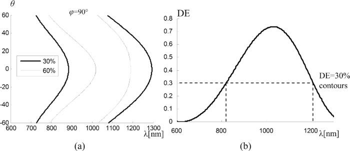

The hologram diffraction efficiency is less sensitive to the out-of-plane angles of incidence (φ = 90 deg) than the in-plane case. As a result, the out-of-plane acceptance angle is much broader than the in-plane.

Overlap of diffraction efficiency from cascaded gratings in the incident range usually does not introduce cross-coupling losses. However, overlapping grating diffraction efficiency in the diffraction range does imply cross-coupling. Cross-coupling results when the diffraction angle of the first grating matches the diffraction angle of the second grating. In this case, the second grating diffracts this ray at a small angle that does not reach the PV cell surface [Fig. 7]. This results in a loss in module output power.

Fig. 7

(a) Nontracking HPC with two holograms and (b) 2-D DE plot. DE = 30% contours are shown. The two holograms H1 and H2 have overlaps in both the incident range and diffraction range.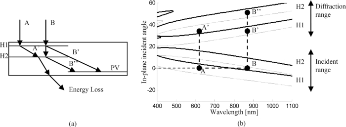

For an HPC with fixed seasonal tilt angle, two holograms can capture most of the incident solar energy throughout the year. In Fig. 7, the combined diffraction efficiency of the two gratings in the incident range covers almost twice the wavelength range of a single grating. However, overlapping DE in the diffraction range indicates that cross-coupling and corresponding reduced output power.

However, overlapping regions of diffraction efficiency in the incident range, as indicated in Fig. 7, does not imply energy losses. For example, the incident ray B is within both H1's and H2's incident range. It is partly diffracted by both H1 and H2 into rays B^′ and B^″ and reach the PV cell area without energy loss.

The cascaded hologram design can be improved with the configuration shown in Fig. 8. The two gratings diffract light in different directions and reduce cross-coupling losses. This extends both the incident angle (±20 deg) and spectral range for the system.

Fig. 8

(a) Optimal design of nontracking HPC with two holograms and (b) 2-D DE plot.

4.2.

One-Axis Tracking Holographic Planar Concentrator Design

For nontracking HPC systems, the acceptance angle must be relatively large to cover daily and seasonal movements of the sun. For a single-axis tracking HPC, this requirement is significantly reduced because another degree of freedom is available to maximize energy collection.

In the nontracking HPC system shown Fig. 9, the out-of-plane direction (hologram fringe direction in Fig. 9) aligns with the daily motion of the sun. However, for the single-axis tracking HPC system in Fig. 9, the tracker follows the sun's daily movement and the out-of-plane direction is aligned with the seasonal solar movement.

Fig. 9

Difference between a nontracking HPC system and a single-axis tracking HPC system.

A design of a single-axis tracking HPC system using three cascaded gratings is shown in Fig. 10. The hologram-to-PV-area ratio (A_H/A_PV) is selected to be 1:1, which implies half the module's PV area is replaced by holographic gratings. This configuration has a 2X geometrical concentration.

Fig. 10

Component layout in a unit cell of a one-axis tracking HPC module. A module is formed by repeating the unit cell. Monofacial PV cells are positioned near the bottom of the module for good optical efficiency.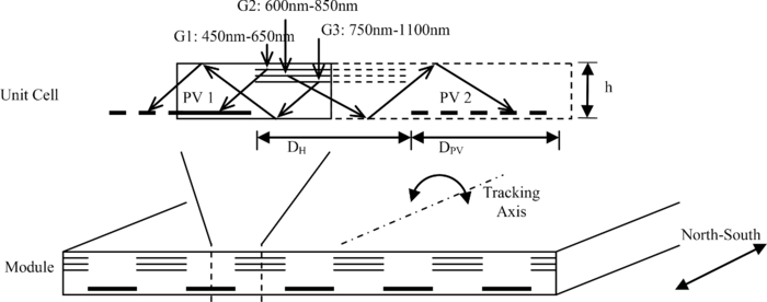

The height ratio H is defined as the height of the module versus the PV cell width (H = h/D_PV). At a fixed hologram-to-PV-cell width ratio of 1:1, the parameter H will influence the optimum grating diffraction angles. If the module is too thin (H < 0.5), then diffracted rays must undergo several total internal reflections to reach the PV cell and increase cross-coupling losses. The result of our simulation shows that an optimum height ratio for a three-grating HPC with D_PV = D_H is 0.7.

Numerical optimization can be used to reduce cross-coupling between gratings that results as an overlap of diffraction efficiency in the diffraction range. However, a small overlap between the diffraction efficiency of G1 and G3 (Fig. 11) is difficult to avoid because these gratings diffract light in the same direction (Fig. 10). This reduces the optical efficiency by ∼5% in the wavelength range from 400 to 600 nm, as shown in Fig. 12.

Fig. 11

Construction parameters for the three gratings in the one-axis tracking HPC design.

Fig. 12

Simulation result of spectral optical efficiency of a one-axis tracking HPC unit cell at normal incidence.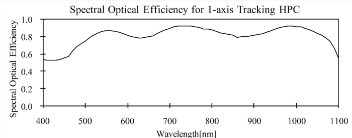

2-D DE plot of the one-axis tracking HPC design in Table 1. (1) Overlaps of diffraction efficiency in the “diffraction range” indicate cross-coupling losses. (2) Diffraction efficiency overlaps in “incident range” do not imply losses.

Table 1

Grating	Construction	Construction	Thickness	Refractive index
No.	angles (deg)	wavelength (nm)	(μm)	modulation
G1	3.5, 50		2.0
G2	–9, –40	488	2.5	0.1
G3	15, 42		4.0

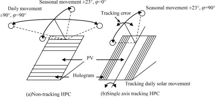
An ideal single N-S axis tracker follows the daily movement of the sun and maintains the in-plane incident angle at θ = 0 deg. The angular bandwidth in the out-of-plane direction is sufficient to cover the seasonal angle variation of the sun throughout the year. The diffraction efficiency of G1–G3 are optimized for maximum diffraction efficiency with θ = 0 deg to improve capture of the sun's illumination spectrum when the tracker maintains the HPC surface directed toward the sun. The tracking error decreases the optical efficiency of the HPC module, as described in Sec. 5.

5. Characterisitcs of One-Axis Holographic Solar Concentrator

5.1.

Spectral Optical Efficiency and Tracking Tolerance

When illuminated on axis, a holographic stack can diffract over a large spectral range corresponding to the spectral response range of many types of PV cells. The spectral performance of the hologram primarily depends on the in-plane angle of incidence. At ±6 deg from the hologram surface normal along the in-plane axis, the overall optical efficiency is 90% of the value at normal incidence. At an in-plane incident angle of ±16.5 deg, the one-axis tracking HPC system still has 80% of the maximum optical efficiency (Fig. 13).

Fig. 13

Simulated optical system efficiency as a function of the incident angle for (a) in-plane and (b) out-of-plane directions. The in-plane direction is also the tracker rotation direction. (1) 10% reduction in optical efficiency with a 6-deg tracking error. (2) 20% reduction in optical efficiency with a 16.5-det tracking error. (3) Annual range of out-of-plane incident angle on a polar one-axis tracker tilted at the latitude angle. (4) Annual range of out-of-plane incident angle for a horizontal tracker installed at the latitude angle (32 deg).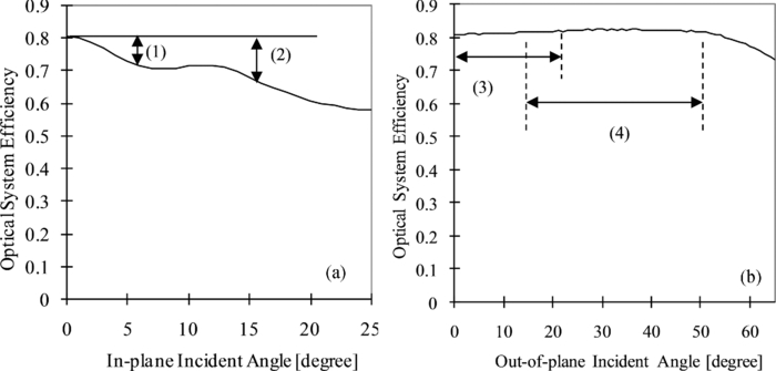

Current one-axis tracking systems can maintain 0.5-deg tracking accuracy using a sensor and feedback system.¹⁵ The one-axis tracked HPC modules have a ±6-deg tracking tolerance. The nontracking acceptance angle of 65 deg is more than sufficient to accommodate the ±23-deg seasonal variation in the sun angle. The larger tolerance and acceptance angle allows much simpler and less costly one-axis tracking systems to be used.

5.2.

Irradiance Nonuniformity

Nonuniform illumination on the PV cell surface can lead to increased series resistance, resulting in decreased fill factor and PV cell efficiency. It has been shown that small irradiance variations have a negligible effect on solar cell efficiency.^{8, 9, 10, 11, 12, 13, 14}

The effect of irradiance variation on the PV cell performance was investigated using nonsequential ray tracing from the hologram aperture to the PV cell surface, as described in Sec. 3.2. It was found that variation in the x direction (along the fringe planes of the hologram) vary much less than in the y direction. Therefore, the variation in irradiance along the x direction was averaged and is plotted as a function of the relative position in the y direction along the cell surface. This was performed for several in-plane angles of incidence. The results for 0 deg (normal incidence) and 55 deg relative to the normal are shown in Fig. 14 and indicate that the irradiance varies by ∼20% over the cell surface. Using this result in Eq. 18 gives a fill-factor derating factor D_f > 98%. Therefore, irradiance nonuniformity results in a relatively small change in HPC performance.

Fig. 14

Simulation result for irradiance uniformity on PV cell. Plotted are normalized irradiance distributions in the y direction (Fig. 1).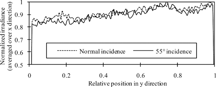

6. Annual Energy Yield Comparison

The performance of six different PV systems under direct normal radiation is compared in terms of daily and annual energy yield per unit module area. The efficiency of PV cells used in all systems is 20% and assumed to be constant over the operating irradiance and temperature range.

Two fixed-tilt modules are simulated, a fully PV-cell-populated module and a nontracking HPC module with 1:1 hologram-to-PV-cell area ratio. The nontracking HPC modules follow the same design as in Ref. 8, which incorporated two hologram layers and achieves an average of 70% optical efficiency. Both fixed modules are installed facing due south at a tilt angle equal to the latitude. The single-axis tracking HPC design in Table 1 and a fully populated PV counterpart are modeled with horizontal and polar one-axis tracking. The horizontal one-axis tracker rotates around a horizontal N-S axis, and the polar one-axis tracker rotates about an axis inclined at the latitude angle in the N-S direction (Fig. 15). All single-axis trackers are considered ideal. An optical efficiency of 95% is assumed for the nonholographic systems. The optical efficiencies of three HPC systems are simulated with the method described in previous sections.

Fig. 15

Module layout, from left to right: (1) fully populated PV modules and nontracking HPC modules (Ref. 8), installed facing due south, at a tilt angle equal to the latitude angle. (2) Single-axis tracking HPC and fully populated PV module on horizontal N-S single-axis trackers. (3) Polar one-axis tracking with flat-panel PV module and one-axis tracking HPC module. The tilt angle is equal to latitude (32 deg).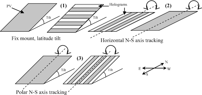

The power generation rate throughout the year is evaluated at 3-min intervals. The daily and annual energy yield is derived by numerical integration of the power generation rate for the corresponding amount of time. The daily energy yield for all six systems is compared in Fig. 16, and the annual energy yield is summarized in Table 2.

Table 2

Annual energy yield comparison, corresponding to the daily energy yield plots shown in Fig. 16.

			(2) Horizontal
System	(1) Fixed tilt		one-axis		(3) Polar one-axis
Type	PV	HPC	PV	HPC	PV	HPC
Annual Yield (kW-h/m²)	401.5	310.7	505.9	426.0	530.7	446.9
Relative to (1)-HPC (%)	129.2	100	162.8	137.1	170.8	143.8
Relative to (3)-PV (%)	75.7	58.5	95.3	80.3	100	84.2

Fig. 16

Daily energy yield as a function of annual day number for HPC and flat-panel PV systems with and without tracking. The integrated annul energy yield is shown in Table 2.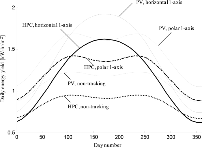

The result shows that the one-axis polar axis tracking HPC system can provide 84.2% of the energy yield provided by a one-axis polar tracking fully populated module. In addition, polar one-axis tracking HPC systems produces 43.8% more energy annually compared to nontracking HPCs due to higher overall module optical efficiency and higher levels of irradiance available to tracking surfaces.

7. Conclusion

A method to design and analyze holographic solar concentrators with single-axis tracking is demonstrated. By using three cascaded optimized holographic diffraction gratings, a broad spectrum (400–1100 nm) can be concentrated onto a PV cell surface. A comprehensive optical system simulation method was developed for single-axis tracking HPC systems. The diffraction efficiency and optical efficiency was measured for an experimental holographic grating formed in dichromated gelatin, and the results are in good agreement with the optical system simulation.

Simulation of an optimized one-axis tracking HPC design showed that 80% optical efficiency at 2X geometric concentration ratio can be achieved with good irradiance uniformity (<20%). The acceptance angle for an optimum HPC configuration is ±65 deg in the nontracking direction and ±6 deg in the tracking direction. An error of ±16 deg in the tracking direction is sufficient to maintain 80% of the maximum optical efficiency.

Daily and annual energy yield is modeled for HPC modules and fully PV-cell-populated modules, with different tracking modes, such as fixed tilt nontracking, horizontal N-S one-axis tracking and polar one-axis tracking. Results of polar one-axis tracking HPC indicate 43.8% increase in annual energy yield per unit area over nontracking HPCs.

Acknowledgments

The authors acknowledge the support of the National Science Foundation (Grant No. 0925085) and the Science Foundation Arizona (Grant No. 443831) for this work.

Appendices

Appendix: Derivatiion of Equations

The single-axis tracking module rotates around a tilted axis in the xz plane (Fig. 17). The tilt angle α is the angle between the rotation axis and the x-axis. The rotation angle β_t is the angle change of the module surface normal [TeX:] $\vec n$ $\vec{n}$ relative to its position at solar noon. The tracking module normal vector is

[TeX:] \documentclass[12pt]{minimal}\begin{document}\begin{equation} \vec n = \left[ {\begin{array}{*{20}c} {\cos \beta _{\rm t} \,\,\sin \alpha } \\[7pt] {\sin \beta _{\rm t} } \\[7pt] {\cos \beta _{\rm t} \,\,\cos \alpha } \\[5pt] \end{array}} \right]. \end{equation}\end{document}

\vec{n} = [\begin{matrix} \cos β_{t} \sin α \\ \sin β_{t} \\ \cos β_{t} \cos α \end{matrix}] .

The direction vector of the sun [TeX:] $\vec n_{\rm S}$

{\vec{n}}_{S}

is represented with the solar azimuth angle θ_ZS and zenith angles ψ_Z relative to the ground surface normal,

[TeX:] \documentclass[12pt]{minimal}\begin{document}\begin{equation} \vec n_{\rm S} = \left[ {\begin{array}{*{20}c} {\sin \theta _{{\rm ZS}} \,\,\cos \psi _{\rm Z} } \\[7pt] {\sin \theta _{{\rm ZS}} \,\,\sin \psi _{\rm Z} } \\[7pt] {\cos \theta _{{\rm ZS}} } \\[5pt] \end{array}} \right], \end{equation}\end{document}

{\vec{n}}_{S} = [\begin{matrix} \sin θ_{ZS} \cos ψ_{Z} \\ \sin θ_{ZS} \sin ψ_{Z} \\ \cos θ_{ZS} \end{matrix}],

and [TeX:] $\vec n_e$

{\vec{n}}_{e}

is the unit vector for the direction corresponding to φ = 0 deg relative to the module

[TeX:] \documentclass[12pt]{minimal}\begin{document}\begin{equation} \vec n_e = \left[ {\begin{array}{*{20}c} { - \sin \beta _{\rm t} \,\,\sin \alpha } \\[7pt] {\cos \beta _{\rm t} } \\[7pt] { - \sin \beta _{\rm t} \,\,\cos \alpha } \\[5pt] \end{array}} \right]. \end{equation}\end{document}

{\vec{n}}_{e} = [\begin{matrix} - \sin β_{t} \sin α \\ \cos β_{t} \\ - \sin β_{t} \cos α \end{matrix}] .

The zenith angle θ and azimuth angle φ relative to the module can be calculated as follows:

[TeX:] \documentclass[12pt]{minimal}\begin{document}\begin{equation} \theta = \cos ^{ - 1} (\mathord{\rightharpoonup \over n} \cdot \mathord{\rightharpoonup \over n} _{\rm S}), \end{equation}\end{document}

θ = \cos^{- 1} (\overset{⇀}{n} \cdot {\overset{⇀}{n}}_{S}),

[TeX:] \documentclass[12pt]{minimal}\begin{document}\begin{equation} \varphi = \cos ^{ - 1} (\mathord{\rightharpoonup \over n} _e \cdot \mathord{\rightharpoonup \over n} _t)\,,\quad \mathord{\rightharpoonup \over n} _t = \mathord{\rightharpoonup \over n} _{\rm S} - (\mathord{\rightharpoonup \over n} \cdot \mathord{\rightharpoonup \over n} _{\rm S})\mathord{\rightharpoonup \over n}. \end{equation}\vspace*{-15pt}\end{document}

ϕ = \cos^{- 1} ({\overset{⇀}{n}}_{e} \cdot {\overset{⇀}{n}}_{t}), {\overset{⇀}{n}}_{t} = {\overset{⇀}{n}}_{S} - (\overset{⇀}{n} \cdot {\overset{⇀}{n}}_{S}) \overset{⇀}{n} .

Fig. 17

Angle conventions for the zenith angle and azimuth angle relative to the tracking surface.

References

1.

S. Abdallah, “The effect of using sun tracking systems on the voltage-current characteristics and power generation of flat plate photovoltaics,” Energy Convers. Manage., 45 1671 –1679 (2004). http://dx.doi.org/10.1016/j.enconman.2003.10.006 Google Scholar

2.

W. C. Dickinson, “Annual available radiation for fixed and tracking collectors,” Sol. Energy, 21 249 –251 (1978). http://dx.doi.org/10.1016/0038-092X(78)90030-0 Google Scholar

3.

S. Nann, “Potentials for tracking photovoltaic systems and V-troughs in moderate climates,” Solar Energy, 45 385 –393 (1990). http://dx.doi.org/10.1016/0038-092X(90)90160-E Google Scholar

4.

J. M. Gordon and H. J. Wenger, “Central-station solar photovoltaic systems: Field layout, tracker, and array geometry sensitivity studies,” Solar Energy, 46 211 –217 (1991). http://dx.doi.org/10.1016/0038-092X(91)90065-5 Google Scholar

5.

R. Winston, J. Minãno, P. Benitez, N. Shatz, and J. C. Bortz, Nonimaging Optics, 18 –22 Academic Press, Burlington (2005). Google Scholar

6.

C. G. Stojanoff, “Review of the technology for the manufacturing of large-format DCG holograms for technical applications,” Proc. SPIE, 3011 267 –278 (1997). http://dx.doi.org/10.1117/12.271375 Google Scholar

7.

J. M. Russo, J. E. Castillo, E. D. Aspnes, G. Rosenberg, and R. K. Kostuk, “Daily and seasonal performance of angularly dependent fixed mount dual aperture holographic planar concentrator photovoltaic modules,” Proc. SPIE, 7769 77690D (2010). http://dx.doi.org/10.1117/12.861950 Google Scholar

8.

J. M. Castro, D. Zhang, B. Myer, and R. K. Kostuk, “Energy collection efficiency of holographic planar solar concentrators,” Appl. Opt., 49 858 –870 (2010). http://dx.doi.org/10.1364/AO.49.000858 Google Scholar

9.

J. E. Castillo, J. M. Russo, G. A. Rosenberg, D. Zhang, and R. K. Kostuk, “Low holographic concentration effects on CIGS,” Proc. SPIE, 7769 77690L (2010). http://dx.doi.org/10.1117/12.862038 Google Scholar

10.

J. Goodman, Introduction to Fourier Optics, McGraw-Hill, New York (1996). Google Scholar

11.

H. Kogelnik, “Coupled wave theory for thick hologram gratings,” Bell Syst. Tech. J., 48 (9), 2909 –2947 (1969). Google Scholar

12.

A. Luque and S. Hegedus, Handbook of Photovoltaic Science and Engineering, Wiley, Hoboken, NJ (2003). Google Scholar

13.

B. Meinel and M. P. Meinel, Applied Solar Energy, Addison-Wesley, Reading, MA (1976). Google Scholar

14.

P. Benítez and J. Miñano, “Concentrator optics for the next-generation photovoltaics,” Next Generation Photovoltaics, Taylor & Francis, New York (2003). Google Scholar

15.

S. A. Kalogirou, “Design and construction of a one-axis sun-tracking system,” Solar Energy, 57 465 –469 (1996). http://dx.doi.org/10.1016/S0038-092X(96)00135-1 Google Scholar

Biographies and photographs of the authors not available.

Citation Download Citation

Deming Zhang, Jose M. Castro, and Raymond K. Kostuk "One-axis tracking holographic planar concentrator systems," Journal of Photonics for Energy 1(1), 015505 (1 January 2011). https://doi.org/10.1117/1.3590943

Published: 1 January 2011

Access the abstract

JOURNAL ARTICLE
18 PAGES

DOWNLOAD PAPER SAVE TO MY LIBRARY

GET CITATION

CITATIONS

Cited by 24 scholarly publications.

Explore citations on Lens.org

RIGHTS & PERMISSIONS

Get copyright permission Get copyright permission on Copyright Marketplace

KEYWORDS

Solar cells

Diffraction

Holograms

Holography

Holographic concentrators

Solar concentrators

Solar energy

Show All Keywords

CHORUS Article. This article was made freely available starting 01 January 2012

1.

Introduction

2.

Holographic Planar Concentrator System Overview