
|
|
1.Introduction to Spectrum SplittingShockley and Queisser have shown that single junction photovoltaic (PV) cells are limited to an efficiency of 33%.1 This limitation stems from the mismatch between the photon energy of the incident solar illumination and the bandgap energy of the PV cell. In order to overcome this limit, multiple bandgap PV cells can be used either in tandem or in parallel to improve the match with the incident solar spectral distribution. In the past, considerable effort has been given to tandem multijunction PV cells that are used in conjunction with a large aperture, high concentration optical element. Although successful, tandem multijunction cells are limited by the requirement of precise lattice matching between different bandgap layers and current matching limitations imposed by the least efficient PV cell. An alternative multijunction configuration uses optics to spectrally separate the incident solar illumination and distribute different spectral bands to single bandgap PV cells with a high response to the separated spectral component.2 The PV cells are spatially separated allowing dissimilar materials (with different lattice constants) to be used and avoids the need for current matching the output from different cell types. Spatial separation of the PV cells increases the freedom of selection of materials by removing the lattice matching requirement (when compared to tandem multijunction cells). On the other hand, the spatial separation and the addition of the optical system make the overall configuration and fabrication more complex. 1.1.Spectral Conversion Efficiency AnalysisWhen a PV cell is used in a spectrum splitting system (SSS), the spectral response of the filters used to separate different spectral bands must be included in the conversion efficiency expression. The filtered efficiency of the ’th PV cell of an SSS can be expressed as where SR, , and FF are the spectral responsivity, open circuit voltage, and fill factor, respectively, and are the parameters of the PV cell.3,4 The incident illumination characteristics are given by the spectral irradiance and the integrated irradiance .5 From the equation above, the spectral conversion efficiency (SCE)4 is given by: . The wavelength-dependent filter transmittance function, , allows for filter characteristics to be used in determining the efficiency of the multiple bandgap PV system. For a system with different PV cells, the total SSS efficiency is given by the following equation:6The total efficiency of the SSS () is equivalent to the optical-to-electrical conversion efficiency reported in the literature for different SSSs (as summarized by Mojiri et al.7). The spectral conversion efficiency analysis for different spectrum splitting configurations is discussed in detail by Russo et al.8 2.Dispersive Spectrum Splitting DefinitionsIn dispersive SSSs, spectral separation is achieved by means of diffraction or refraction by one or more optical elements.6,9–11 The magnitude of the dispersion depends on the type of component used and can be expressed as a dispersion factor .8 When a dispersive filter is illuminated with the solar spectrum (i.e., AM1.5), each wavelength is dispersed into a continuum of wavelengths spatially separated along the receiver plane.8 In this paper, we quantify the degree to which the spatially dispersed spectrum on the receiver plane is matched to the position, size, and responsivity of a PV cell with the spectral overlap function . Insufficient spectral separation results in the projection of the system aperture with an overlap of wavelengths on the receiver plane. The incomplete separation of wavelengths on the receiver plane as shown in Fig. 1(a) results in spectral mismatch losses between the separated spectral components and the PV cell spectral responsivity. Fig. 1(a) A single dispersive filter projects the complete spectrum along the receiver plane (). Wavelength separation only occurs at the edge of the aperture. (b) Focusing power is combined with the dispersive element. The geometrical parameters for the cross-correlation analysis are shown. 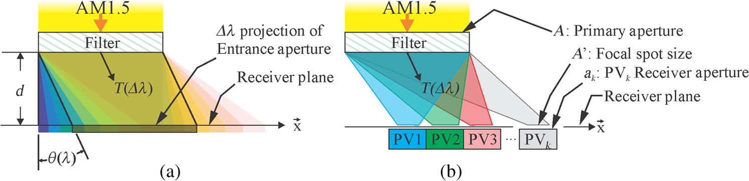 In order to include dispersion effects in the calculation of the efficiency, Eq. (1) must include a spectral overlap function for each PV cell. These functions are the result of the spatial cross-correlation of the wavelength distribution as a function of position and the spatial aperture function of the cells on the receiver plane. The total efficiency of an SSS using a dispersive optical element with different PV cells can be calculated using the following equation: where is the transmittance (or efficiency for diffractive optical elements) of the filter and is the overlap function for the ’th PV cell. The value of the ’th overlap function at each wavelength is the fraction of the energy incident at the receiver plane that is collected by the aperture of the ’th PV cell. As shown in Eq. (3), each PV cell () has a distinct overlap function, , associated with it.Depending on the type of PV cells that comprise the SSS, there will be an optimum spectral range for each cell such as The optimum range for a combination that includes a GaAs,12 ,13 and silicon14 PV cell is shown in Fig. 2. The fraction of incident light in the range that is collected by the ’th PV cell can be calculated as where is the optical transfer efficiency of the aperture of PV ’th cell. Ideally, a system for maximum collection () will be designed to have in the range for a specific PV cell and outside of it as shown in Fig. 2.Fig. 2(a) Optimum receiver axis with photovoltaic (PV) cell size and position parameters shown for (blue), GaAs (red), and Si (black) as given by the optimum spectral range (b) for a diffraction grating () with ideal overlap functions. Equation (7) was used to convert from position (a) to wavelength (b). 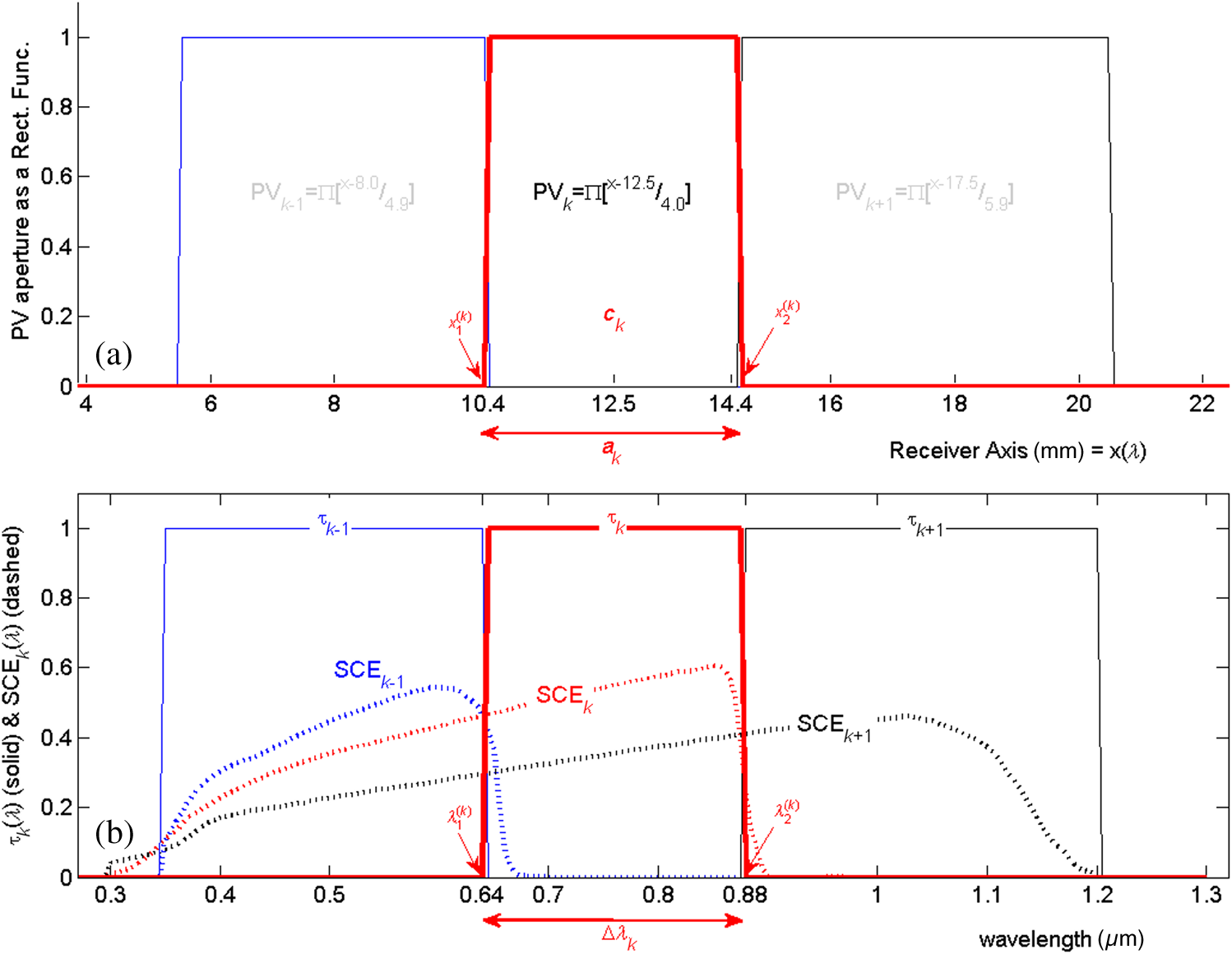 2.1.Dispersion and Geometrical ParametersThe spectral overlap function will depend on the dispersion and geometrical parameters of the SSS listed in Table 1 and shown in Fig. 1. Table 1Dispersion and geometrical parameters used to calculate the spectral overlap function.
2.1.1.DispersionThe dispersion factor is given by8 where is the dispersion angle from the filter in the medium between the filter and the receiver plane as shown in Fig. 1. The magnitude of the dispersion factor is a function of the type of dispersive element used (prism, diffraction grating, etc.). The position of a particular wavelength, , within the continuum of dispersed wavelengths can be calculated using where is the separation distance between the dispersive filter and the receiver plane.2.1.2.System aperture, spot size, and focusingFor systems without secondary optics,10 the receiver parameters (position and aperture) refer to the aperture of the PV cell itself. For systems with a secondary optic (such as a homogenizer,15 lens, or compound parabolic concentrator6,16,17) the receiver parameters refer to the position and size of the entrance aperture of the secondary optic. In this paper, we define focusing power as the ratio of the system entrance aperture () over the RMS spot size () at the receiver plane as shown below: In a concentrating photovoltaic system without spectrum splitting (), the term focusing as defined in this paper is interchangeable with geometrical concentration.182.1.3.Receiver size and positionAlthough the PV cell size and position depends on fabrication and design constraints, the selection of semiconductor materials (their spectral responsivities) will dictate the optimum spectral range defined in Eq. (4) above. It is possible to calculate optimum size and position for each of the PV cells based on the SCE of the cells that comprise the SSS using Eq. (7) to convert the optimum spectral range from wavelengths to positions at the receiver axis using the following equations: The equations above were used to obtain the correspondence between horizontal axes of the two sections of Figs. 2(a) and 2(b). The equations above guarantee that the and wavelength components of the dispersed continuum align with the edges of the ’th PV cell at the receiver plane. The optimum size for a PV cell depends on the separation distance and the dispersion factor as shown in Eq. (9) and Fig. 3. Also shown in Fig. 3 is the fact that as the separation distance, , is reduced, the optimum PV cell aperture, , is also reduced.Fig. 3PV aperture size () versus separation distance (). Increasing the dispersion increases the slope of the graph. 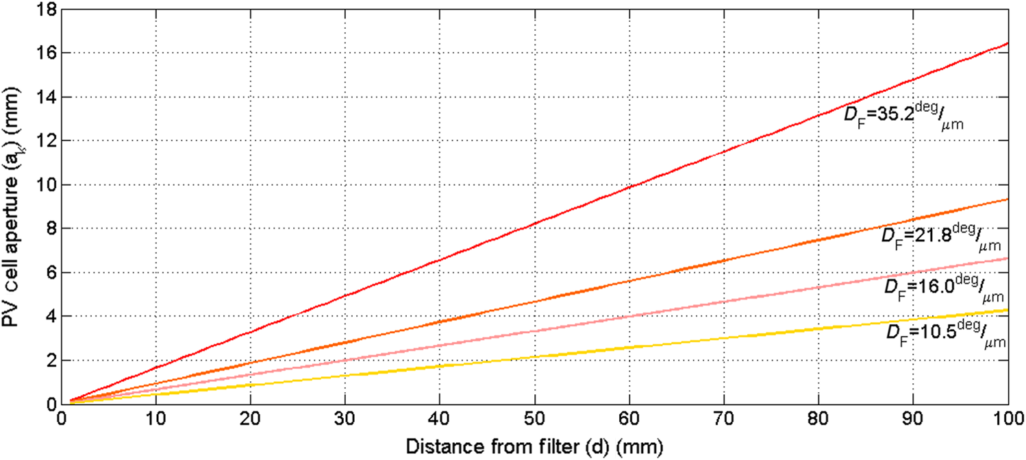 If all dispersed wavelength components, , are focused down to a perfect image point, all the wavelength components in the optimum spectral range are collected by an optimum sized PV cell, the overlap function is ideal (as shown in Fig. 2) and the dispersion losses are zero. However, since the wavelength components have a finite extent, they either overlap completely, partially, or miss the PV aperture giving rise to dispersion loss. This is explained in more detail in Sec. 3.3. 3.Dispersive Cross-Correlation AnalysisIn this section, the spectral components of the dispersed spectrum will be defined as rectangular functions of position. The spectral overlap function will be defined and the dispersion losses will be explained. 3.1.Rectangular Function Representations at the Receiver PlaneAs shown in Fig. 1 and by Videos 1 and 2, the continuum incident at the receiver plane is comprised of consecutive and overlapping wavelength components that have finite extent. The size and separation of the components will depend on the amount of focusing defined in Eq. (8) and the parameters listed in Table 1. It is possible to represent the spectral continuum as a set of rectangular functions positioned along the receiver axis as where the width is a function of the RMS spot size () along the dispersion direction .As shown in Fig. 2, the ’th PV cell can be represented as a rectangular function along the receiver axis as where the width and position of the rectangular function are the size () and displacement () of the PV cell, respectively.3.2.Cross-Correlation Analysis to Obtain the Spectral Overlap FunctionDispersion will cause the wavelength components to have varying degrees of overlap with different PV cell apertures on the receiver plane. A spectral overlap function can be obtained by computing the overlap between functions and the PV cell aperture function for different positions of the dispersed wavelengths as The operation shown in Eq. (12) is equivalent to a cross-correlation19 between the rectangular functions and with a wavelength projection position withThe spectral overlap function can be obtained as a function of wavelength using the equation for from Eq. (7) in Eq. (13). The result of the cross-correlation operation is shown in Fig. 4 (and in Videos 1 and 2) for an equal spot size to PV cell aperture size () and for a spot size 20 times smaller (). This figure shows, as expected, that reducing the RMS spot size relative to the PV cell aperture size results in a more square shape for the spectral overlap function. Fig. 4Overlap functions for (a) and for (b). An animation of the cross-correlation operation shown one wavelength at a time for and for in Videos 1 and 2, respectively (Video 1, MP4, 0.98 MB) [URI: http://dx.doi.org/10.1117/1.JPE.5.1.054599.1] and Video 2, MP4, 0.98 MB) [ http://dx.doi.org/10.1117/1.JPE.5.1.054599.2]. 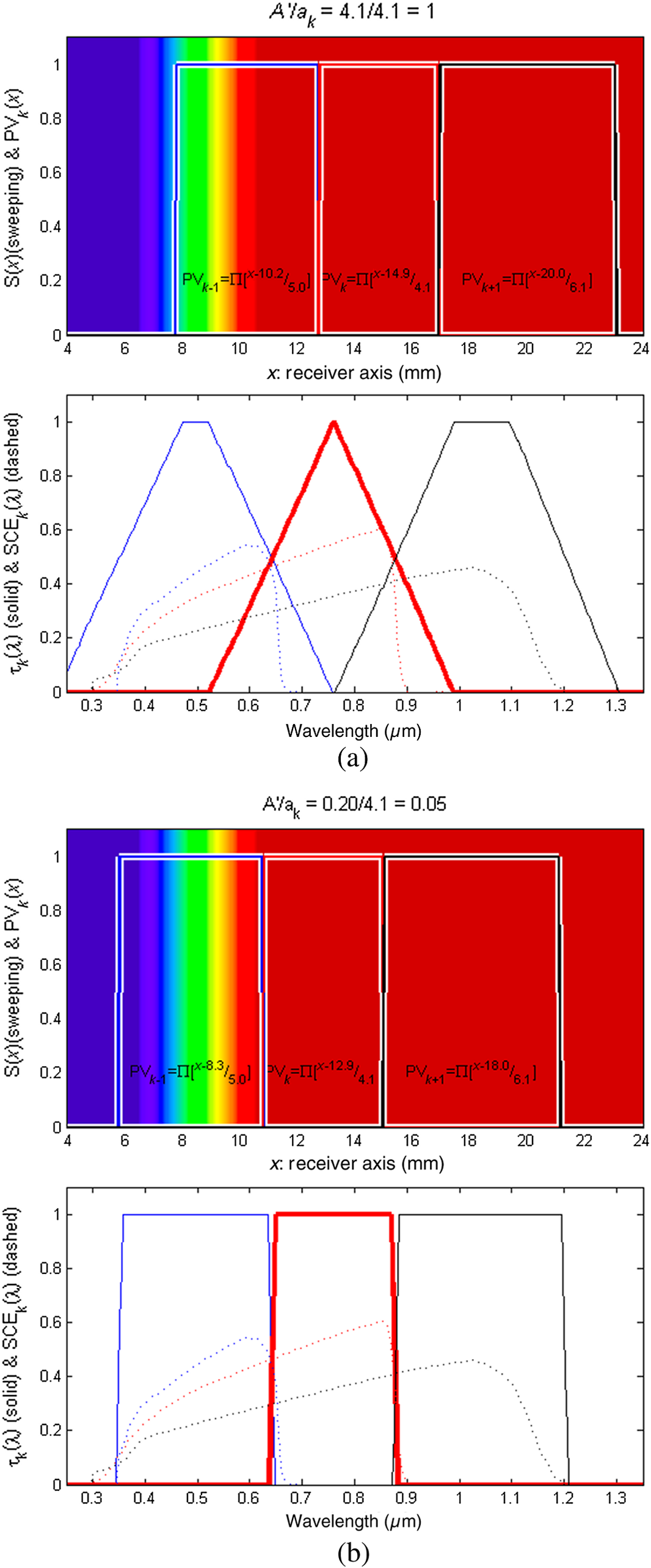 3.2.1.Dispersion losses and aperture transfer efficiencyIncident light can be incident on one or more cells, or miss the apertures of all of the cells (be a loss). Since energy must be conserved, the summation of all spectral overlap functions for each wavelength is Dispersed light that does not illuminate any of the PV cell apertures is a dispersion loss and can be calculated as For the case where the summation term in Eq. (15) is equal to zero (as in Fig. 5 where for and ), the dispersed light misses all the cells in the system at that wavelength range and is completely lost due to dispersion. If the summation term in Eq. (15) is less than one [as in Fig. 5 where for and ], some of the light at that wavelength is incident on one or more PV cells and some of it is lost due to dispersion. Finally, if the summation term is equal to one [as in Fig. 5 where for ], all of the light is incident on one or more PV cells and there is no aperture loss. Note that a value larger than one for the summation term would indicate more energy at the receiver axis than at the entrance aperture and is invalid since it violates energy conservation.Fig. 5Spectral overlap functions for a system using (blue), GaAs (red), and Si (black) with aperture and spatial crosstalk losses highlighted. The optimal spectral range is highlighted for GaAs. 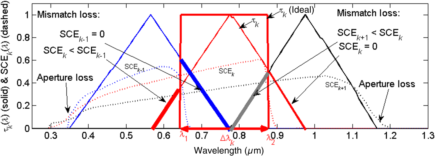 In an SSS, PV cells that are not properly matched with the incident spectrum will incur thermalization losses below and will not be absorbed above similar to a broadband PV system. Figure 5 shows ideal and nonideal overlap functions for a GaAs PV cell (in red). The nonideal overlap function extends beyond and does not completely fill the optimal wavelength range (as shown in Fig. 5). The extension of the overlap function beyond its corresponding range is defined as a mismatch loss in this paper. These losses are proportional to the difference between the ’th (mismatch cell) SCE and the maximum possible SCE of the system and can be calculated as where the SCEs are a functions of wavelength. The equation above is equal to zero in the optimal spectral range since is matched and maximum. At wavelengths corresponding to energies below the bandgap energy, and the mismatch loss is maximum. In Fig. 5, it can be seen that for the same range that has zero aperture loss , some light is incident on the PV cell (highlighted in blue) and PV cell (highlighted in gray). The mismatch losses in this example are proportional to (where ) and (where ), respectively, and are both negative.The dispersion loss terms defined in this section [in Eqs. (15) and (16)] quantify the amount the overlap function deviates from ideal conditions and affects the overall efficiency of the SSS. Using these loss definitions, consider the efficiency of the system in the absence of dispersion losses as 3.3.Form Factor: Spectral Shape of the Overlap FunctionIn Eq. (12) with (equal spot size and aperture size), only a narrow spectral band will be collected completely [] by the PV cell. This is indicated by the triangular spectral shape of the overlap functions in Fig. 5 where at the peaks of each function. In Fig. 5, for the rest of the wavelength components due to a mix of the aperture and mismatch losses defined in the previous section. As shown in Fig. 6(a), when the spot size and the PV aperture size are equal, all the wavelength components of the continuum preceding and subsequent to the peak only partially overlap with the PV cell aperture, hence the overlap function value and only a part of the matched spectrum is collected. Fig. 6Spectral overlap function for a form factor of (a) unity and (b) four. Above, overlapping projections shown for (a) two and (b) three wavelengths. The spatial crosstalk due to incomplete separation is highlighted for both cases. 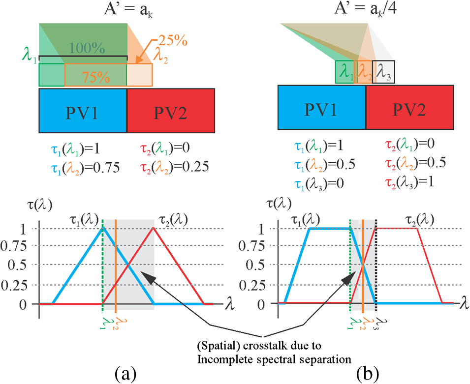 Changing the relationship between the spot size and the PV aperture to by incorporating focusing () in the collection aperture, the width of the spectral band captured by the cell increases. This case is shown in Fig. 6(b), where and the overlap function has a trapezoidal shape as a function of wavelength. Assuming that the geometry of the system allows for , the spectral overlap function can approximate a square shape. Another useful parameter in specifying an SSS is the form factor defined as The form factor is analogous to specifying a spatial frequency of the SSS in terms of how many of the dispersed spectral projections and what proportion fit in the aperture of each PV cell. In this context, the energy collection efficiency can be considered as the transfer efficiency of the aperture of the ’th PV cell compared to a system with no dispersion losses (ideal spectral overlap function). The case where there are no dispersion losses corresponds to 100% transfer efficiency. The “transfer efficiency” can be used to determine the amount of focusing power () required to achieve a desired amount of energy collection efficiency for an SSS with a fixed collection aperture () and PV cell aperture size (), for example, when results in an energy collection efficiency of (for an optimally sized PV cell) as defined in Eq. (5). If the ratio of , a focusing power of is required to achieve this collection efficiency. Reducing the form factor to values much less than increases the aperture transfer efficiency to values close to unity and reduces the dispersion losses to a minimum. This effect can be seen in Fig. 7, where the optical transfer efficiency of the PV apertures is near 100% with form factor values . Values of correspond to incomplete spectrum separation due to a spot size larger than the PV aperture (). As seen in seen in Fig. 7, the mismatch loss () is much larger than the aperture loss due to the mismatched light that falls on neighboring PV cells. One important conclusion of this analysis is that dispersive spectrum splitting requires form factors of less than unity to have high aperture transfer efficiencies. This implies that focusing power (i.e., concentration) is necessary. This requirement increases the complexity of the system, reduces the acceptance angle,3 and has an effect on the angular distribution and hence the response of the PV cell.20,21 Fig. 7Aperture transfer efficiency (), SSS efficiency () and dispersion loss () as a function of form factor () for optimized cell sizes ( since for the selected cells ). The case where the PV cell size is forced to be equal is expanded in the Appendix. 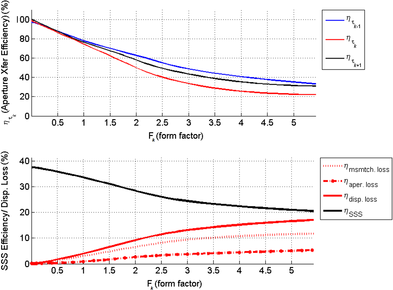 3.3.1.Scaling effectsSince a form factor (as shown in Fig. 7) is required for maximum optical transfer efficiency of the PV cell aperture, a spot size [following Eq. (18)] is also required. When the height of the system () is reduced (Fig. 2) greater focusing power (i.e., smaller ) is required to produce a smaller diffraction limited spot on the receiver plane. Figure 8 shows the required spot size when the separation height ( in Fig. 1) is reduced from 100 to 0.001 mm for a system with a 10-mm aperture. This figure also shows that there is a critical separation distance for this system (near 10 mm at for and smaller for others) below which the optical transfer efficiency is low due to insufficient dispersion. As the system cannot maintain a spot size to sustain , the form factor increases and the transfer efficiency decreases. As shown in Fig. 8, increasing the dispersion increases the transfer efficiency. 4.ConclusionsIn this paper, it was shown that controlling the spatial extent of the spectral distribution is critical for maintaining high energy collection efficiency of transmission type SSSs. The spatial extent of different spectral components that are separated by the dispersive element is controlled using focusing power at the collection aperture of the system. This approach was quantified using a cross-correlation analysis for energy collection efficiency as a function of the form factor of the system that includes the collection and PV cell apertures and the focusing power of the SSS. With the cross-correlation analysis, the spectral overlap function of each PV cell of the SSS was obtained. In this analysis, the losses caused by dispersion were defined as the degree at which the dispersed wavelength components overlapped with the intended PV cell aperture. Dispersion losses were found to be of two types: aperture losses and mismatch losses. Aperture losses were defined as light that does not illuminate the aperture of any PV cell. Mismatch losses are caused by PV cells that are not properly matched with the incident spectrum due to dispersion. It was found that the form factor needs to be minimized in order to maximize the optical transfer efficiency of the PV apertures and minimize the dispersion losses. The cross-correlation analysis was shown to provide a useful method to design dispersive SSSs to minimize dispersion losses, maximize overall system efficiency, and analyze effects of scaling the separation distance between the entrance aperture and the receiver plane (PV cells). Other methods either attribute the dispersion effects or “blurred spectrum” to the angular extent of the solar illumination11 or do not characterize the dispersion losses separately from other optical losses.10 AppendicesAppendix:Nonoptimal Cell SizeMinimizing the form factor increases the optical transfer efficiency to near 100% only for PV apertures with optimum sizes following Eqs. (4) and (9). Design and fabrication constraints may limit the dimensions of the PV cells used (e.g., equal sized PV cells) to sizes that are not optimum. For undersized PV cells [smaller than the optimal size calculated in Eq. (9)], the ideal aperture transfer efficiency will not reach 100%. This is because the spectral bandwidth captured by the cell is smaller than the optimal spectral range. Conversely, for oversized PV cells [larger than the optimal size calculated in Eq. (9)], the spectral bandwidth captured is larger than the optimal spectral range (actually it encompasses it completely). Although the oversized cell can achieve a 100% theoretical aperture transfer efficiency, wavelength components outside of the optimal spectral range captured by the oversized cell will incur in mismatch losses. These losses will limit the aperture transfer efficiency of the neighboring cells to values . In the case shown in Fig. 9, (GaAs) is optimally sized while () and (Si) are not (both are smaller than optimal). Examination of the optical transfer efficiency in Fig. 9 shows that reducing the form factor does not compensate for aperture losses caused by nonoptimally sized cells. This can be seen in the InGaP2 and Si cells reaching a maximum of 70% and 85% optical transfer efficiency, respectively. The optimally sized cell (GaAs) reaches nearly 100% for as expected. Fig. 9Aperture transfer efficiency (), SSS efficiency (), and dispersion loss () as a function of form factor () for equal cell size (). Only the size of the ’th cell has been optimized for its corresponding optimum wavelength range . 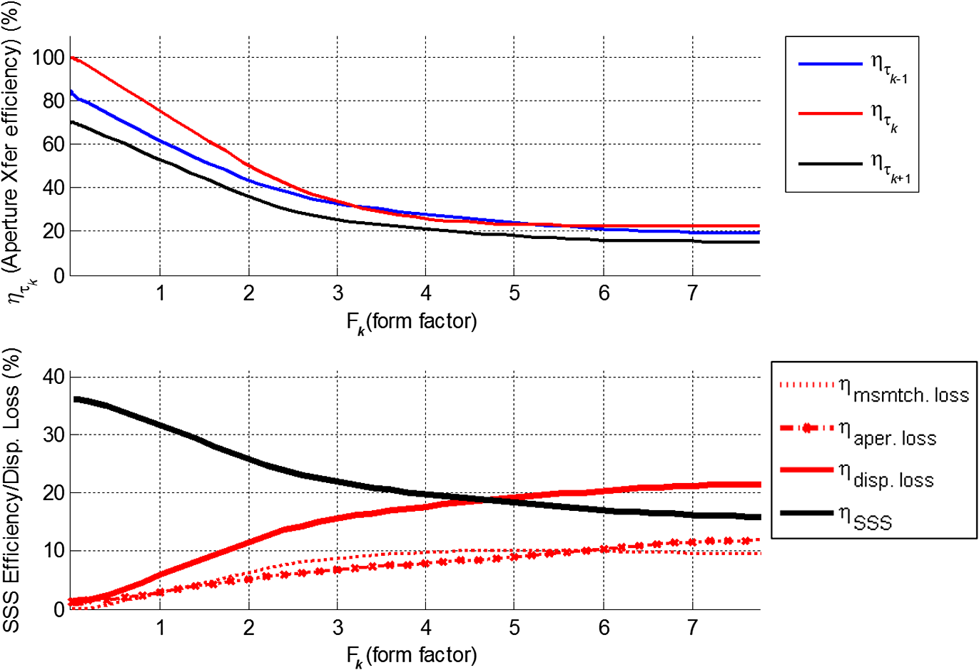 In order to maximize the SSS efficiency , it is important to design the optical system in a way that the most efficient PV cell of the SSS has the highest aperture transfer efficiency when fabricating all PV apertures to be optimally sized is not possible. This is because the is the summation of the filtered efficiencies of the PV cells given in Eq. (2). In the case shown in Fig. 9, the optical system was designed to have maximum aperture transfer efficiency (theoretical 100%) for the most efficient cell of the SSS (GaAs) assuming that all PV apertures were limited to the same dimensions. AcknowledgmentsThe authors wish to acknowledge support from the NSF/DOE ERC cooperative agreement No. EEC-1041895, NSF Grant Nos. 0925085 and 1405619, State of Arizona TRIF (WEES) program and the Research Corporation. ReferencesW. ShockleyH. J. Queisser,
“Detailed balance limit of efficiency of p-n junction solar cells,”
J. Appl. Phys., 32
(3), 510
(1961). http://dx.doi.org/10.1063/1.1736034 JAPIAU 0021-8979 Google Scholar
A. Barnettet al.,
“Very high efficiency solar cell modules,”
Prog. Photovoltaics Res. Appl., 17
(1), 75
–83
(2009). http://dx.doi.org/10.1002/pip.v17:1 PPHOED 1062-7995 Google Scholar
A. LuqueS. Hegedus, Handbook of Photovoltaic Science, 1st ed.John Wiley & Sons Ltd., West Sussex
(2003). Google Scholar
M. HamdyF. LuttmannD. Osborn,
“Model of a spectrally selective decoupled photovoltaic/thermal concentrating system,”
Appl. Energy, 30 209
–225
(1988). http://dx.doi.org/10.1016/0306-2619(88)90046-3 APENDX 0306-2619 Google Scholar
D. R. MyersC. A. Gueymard,
“Description and availability of the SMARTS spectral model for photovoltaic applications,”
Proc. SPIE, 5520 56
–67
(2004). http://dx.doi.org/10.1117/12.555943 PSISDG 0277-786X Google Scholar
J. M. Russoet al.,
“Grating-over-lens concentrating photovoltaic spectrum splitting systems with volume holographic optical elements,”
Proc. SPIE, 8821 882106
(2013). http://dx.doi.org/10.1117/12.2026020 PSISDG 0277-786X Google Scholar
A. Mojiriet al.,
“Spectral beam splitting for efficient conversion of solar energy—a review,”
Renewable Sustainable Energy Rev., 28 654
–663
(2013). http://dx.doi.org/10.1016/j.rser.2013.08.026 RSERFH 1364-0321 Google Scholar
J. M. Russoet al.,
“Spectrum splitting metrics and effect of filter characteristics on photovoltaic system performance,”
Opt. Express, 22
(S2), A528
(2014). http://dx.doi.org/10.1364/OE.22.00A528 OPEXFF 1094-4087 Google Scholar
M. Gordonet al.,
“Planar holographic spectrum-splitting PV module design,”
Proc. SPIE, 8468 846808
(2012). http://dx.doi.org/10.1117/12.929387 PSISDG 0277-786X Google Scholar
M. Stefancichet al.,
“Single element point focus spectral splitting concentrator with CIGS multiple bandgap solar cells,”
Proc. SPIE, 8821 882108
(2013). http://dx.doi.org/10.1117/12.2024386 PSISDG 0277-786X Google Scholar
J. Y. TaudienL. A. Kern,
“Concentrating and spectrum splitting optical device in high efficiency CPV module with five bandgaps,”
Proc. SPIE, 8821 88210A
(2013). http://dx.doi.org/10.1117/12.2024710 PSISDG 0277-786X Google Scholar
M. A. Greenet al.,
“Solar cell efficiency tables (version 39),”
Prog. Photovoltaics Res. Appl., 20
(1), 12
–20
(2012). http://dx.doi.org/10.1002/pip.v20.1 PPHOED 1062-7995 Google Scholar
A. L. Grayet al.,
“Multi-terminal dual junction InGaP2GaAs solar cells for hybrid system,”
in 2008 33rd IEEE Photovoltaic Spec. Conf.,
1
–4
(2008). http://dx.doi.org/10.1109/PVSC.2008.4922575 Google Scholar
J. Zhaoet al.,
“19.8% efficient ‘honeycomb’ textured multicrystalline and 24.4% monocrystalline silicon solar cells,”
Appl. Phys. Lett., 73
(14), 1991
(1998). http://dx.doi.org/10.1063/1.122345 APPLAB 0003-6951 Google Scholar
K. Kreske,
“Optical design of a solar flux homogenizer for concentrator photovoltaics,”
Appl. Opt., 41
(10), 2053
(2002). http://dx.doi.org/10.1364/AO.41.002053 APOPAI 0003-6935 Google Scholar
J. M. Russoet al.,
“Grating-over-lens holographic spectrum splitting concentrating photovoltaics,”
in Renewable Energy Environment,
RW1D.2
(2013). https://doi.org/10.1364/OSE.2013.RW1D.2 Google Scholar
D. Vincenziet al.,
“Concentrating PV system based on spectral separation of solar radiation,”
Phys. Status Solidi, 206
(2), 375
–378
(2009). http://dx.doi.org/10.1002/pssa.v206:2 PHSSAK 0031-8957 Google Scholar
R. J. KoshelI. A. Walmsley,
“Non-edge-ray design: improved optical pumping of lasers,”
Opt. Eng., 43
(7), 1511
–1521
(2004). http://dx.doi.org/10.1117/1.1751400 OPEGAR 0091-3286 Google Scholar
A. Papoulis, The Fourier Integral and its Applications, 244
–245 McGraw-Hill, New York
(1962). Google Scholar
D. Zhanget al.,
“Optical performance of dichroic spectrum-splitting filters,”
J. Photonics Energy, 4
(1), 043095
(2014). http://dx.doi.org/10.1117/1.JPE.4.043095 JPEOBV 1947-7988 Google Scholar
Y. Wuet al.,
“Optical performance of dichroic filters in solar spectrum-splitting application,”
in Renewable Energy Environment,
JM3A.17
(2013). https://doi.org/10.1364/FREEFORM.2013.JM3A.17 Google Scholar
BiographyJuan Manuel Russo received his Bachelor of Science degree in electrical and electronic engineering in the Technological University of Panama in 2004, received a Master of Science in electrical and computer engineering in the University of Arizona in 2007 and is currently pursuing a PhD degree in electrical and computer engineering at the University of Arizona. Also, he has industry experience developing holographic planar concentrator solar modules. His current research interests include optical engineering, holography, illumination, and solar energy. He is a member of SPIE. Shelby Vorndran received her bachelor's degree in physics from DePauw University in 2010. She received a master’s degree in optical science from the University of Arizona in 2013 and is currently pursuing a PhD degree in optical science. In Photonic Systems Laboratory, she designs and fabricates diffractive holographic and surface relief structures to control spectral irradiance. Her current research interest is in renewable energy, specifically photovoltaic, and biofuel systems. Yuechen Wu received his Bachelor of Science degree in electrical and computer science engineering at the University of Toledo in 2012. He is currently pursuing a PhD degree in electrical and computer engineering, and working at the Photonic System Laboratory at the University of Arizona. His research interests include diffractive optics, optical engineering, micro-optics, and solar energy. Raymond K. Kostuk has a joint professor position with UA’s ECE Department and the College of Optical Sciences. He received a PhD degree in electrical engineering from Stanford University. His primary area of expertise is in holographic concepts, materials, and applications, with over 30 years experience in that area. He is a fellow of the Optical Society of America and SPIE. |


